Chapter 1 PART 1 - Basics & Fundamentals
1.1 Programming and Remote Sensing Basics
1.1.1 Remote Sensing Language
A) Definition
The term Remote sensing has been variously defined. Some of its early definitions include:
The art or science of telling something about an object without touching it. (Fischer et al., 1976)
Remote sensing is the acquisition of physical data of an object without touch or contact. (Lintz and Simonett, 1976)
Remote sensing is the observation of a target by a device separated from it by some distance. (Barrett and Curtis, 1976)
The term remote sensing in its broadest sense means "reconnaissance at a distance." (Colwell, 1966)
Thus, in the context of this training, we can define Remote Sensing as the science of acquiring information about a given target, object or phenomenon on the surface of the Earth by sensors on-board various platforms orbiting our planet.
B) Building blocks of remote sensing
Although the many different methods for collection, processing and interpretation of remotely sense data can vary widely, they will always have the following essential components:
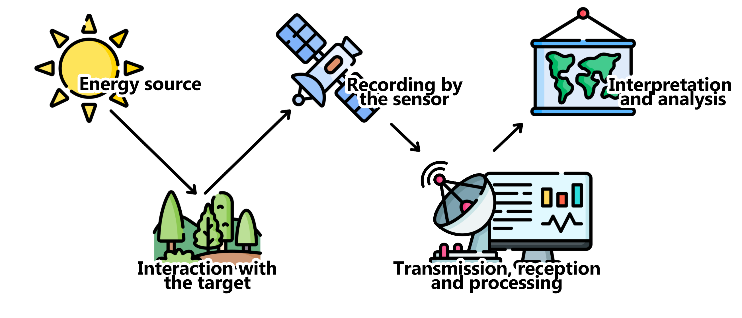
Figure 1.1: Basic components of a remote sensing system.
- Energy Source
The source of the electromagnetic radiation/energy (EMR) is the first requirement of any remote sensing process. The electromagnetic spectrum is used to "classify" the EMR according to its wavelength:
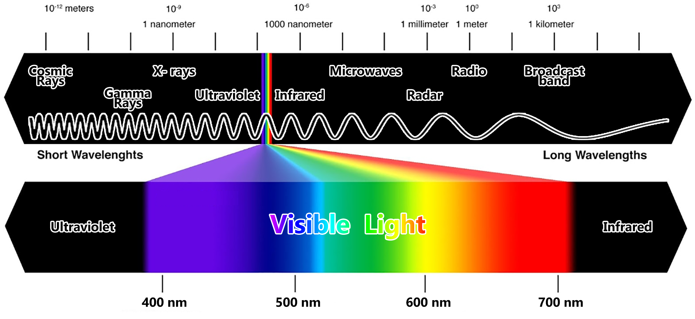
Figure 1.2: The Electromagnetic Spectrum
Depending on the source of energy they are using, the different remote sensing systems can be classified as active or passive. Active sensors will produce its own source of energy for the illumination of the target. They will emit the energy toward the target being investigated and the energy reflected by this target is detected and measured by the sensor. Usually, these sensors operate in the microwave range of the electromagnetic spectrum. On the other hand, passive sensors only measures the energy that is naturally available, usually from the sun. These sensors can only be used to detect the energy being reflected during the time when the sun is illuminating the Earth. These sensors usually measure energy from the optical range (visible, near infrared, short-wave infrared and thermal infrared).
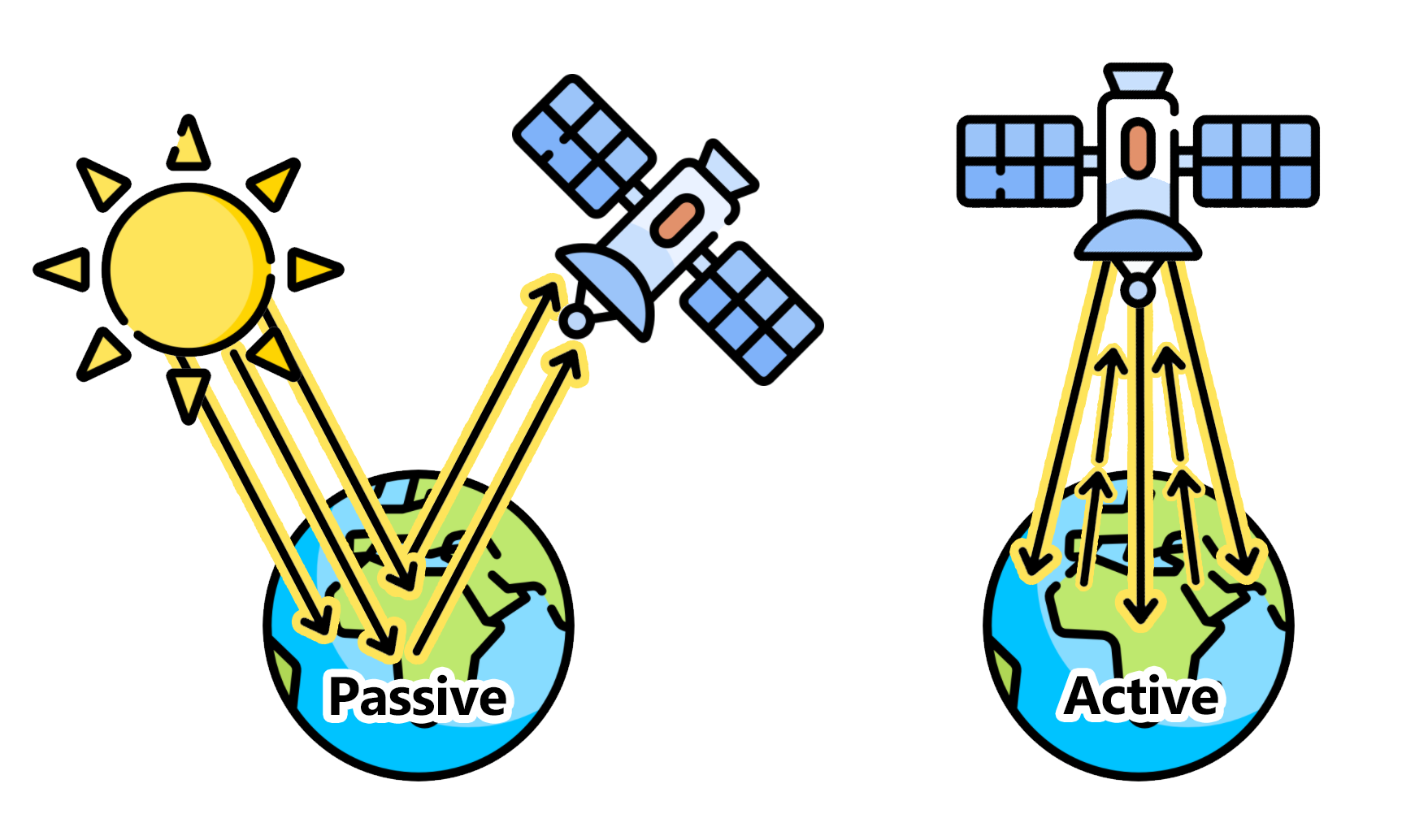
Figure 1.3: Remote sensing can be classified as Passive or Active based on the source of energy.
You can also think about these concepts of active and passive using a handheld photographic camera as an example: When photographing a target in the dark, the camera flash will provide the energy necessary to illuminate the target. Therefore, in that case, the camera is an active sensor. On the other hand, this same camera will be a passive sensor when you are photographing a target or object during the day, when the target being illuminated by sun light and no flash is necessary.
- Interaction with the target/object
The most common medium in between the source and target is the atmosphere. This is where the first interaction occurs. As the EMR travel from its source to the target, it will come in contact with and interact different atmosphere constituents: aerosols, water vapor, solid particles, etc. Secondly, once the EMR makes its way through the atmospherethe to the target, it will interact with it depending on the target properties and energy wavelength. The EMR can have different types of interaction when it encounters matter; whether it is gas, solid or liquid: it can be transmitted (that is, it passes through the target), absorbed (that is, the target absorbs the energy usually increasing its temperature as a result), emitted (that is, energy is emitted from all matter at temperatures above the absolute zero of 0 Kelvins), scattered (that is, deflected in every direction) and reflected (that is, energy bounces off the target's surface and its direction is usually a function of target structure and texture).
Keep in mind: All targets can show different proportions of each of these interactions.
- Recording of the energy by the sensor
The sensor - often onboard of airplanes or satellites in space - will measure the returning EMR after it has interacted with the target and the atmosphere. This measurement is converted into a digital image with discrete values in units of digital number (DN) for each image pixel. Depending on the sensor, these resulting images will have different characteristics (or resolutions). They are:
Spatial Resolution: usually known as pixel size. It refers to the sensor's ability to discriminate different objects/targets. A higher spatial resolution means a smaller pixel size which, in turn, means that smaller objects can be distinguishable as separate targets.
Spectral Resolution: Different sensors will measure the EMR at specific ranges (or wavelengths), usually called bands. Thus, the spectral resolution of a sensor usually refers to the number and bandwith of these bands.
Radiometric Resolution: Usually measured in bits, it refers to the sensor's ability to detect the smallest change in the spectral reflectance among different targets. For example, a 8-bit image will have 256 levels of brightness while a 16-bit image has 65,536 levels of brightness.
Temporal resolution (sensors onboard satellites): is the time required for the satellite to collect two images at the same geographic location on Earth. Higher temporal resolution means less time for revisiting the same location. However, temporal resolution is usually inverselly proportional to spatial resolution: The larger the pixel size, the larger area the sensor will cover which means less time until the next revisit.
- Transmission, Reception, and Processing
The EMR recorded by the sensor is transmitted in an electronic form to a receiving station on Earth where the data is processed and stored.
- Analysis and Interpretation (we are here!)
This is where this training is focused on! The EMR was transformed into a digital dataset where we can use specialized instruments/hardware/software to extract information about the target observed. This extraction is often done through image processing (or digital image processing), which is the process which makes an image interpretable for a given use. There are many methods of image processing, but these are the most common ones:
Image correction: The digital image recorded by the sensor on a satellite (or aircraft) may contain errors related to the geometry and brightness values of the pixels. For example, a geometrical correction, also called geo-referencing, is a procedure where the content of image will be assigned a spatial coordinate system (for example, geographical latitude and longitude).
Image enhancement: This is related to modification of an image, by changing the pixel brightness values, to improve its visual aspects so that the actual analysis of images will be easier, faster and more reliable.
Image classification: The overall goal of this method is to categorize all pixels in an image into themes (or land cover classes). This resulting map with its limited number of classes can be more readily and sucessfully interpreted compared to the raw image and it is often use for planning purposes. There are supervised and unsupervised methods for classification of an image: A supervised classification (human-guided) is based on the idea that a user can select sample pixels in an image that are representative of specific classes and then direct the image processing software to use these training sites as references for the classification of all other pixels in the image. These samples are selected based on the knowledge of the user. On the other hand, an unsupervised classification (computer/software-guided) is where the output classes are based on the software's ability to determine which pixels are related, using several different models and techniques.
This final component of Remote Sensing (V) is achieved when we apply the extracted information to solve a particular problem.
C) Spectral Signatures: A target's spectral fingerprint
As mentioned before, remote sensing is based on the measurement of reflected (or emitted) radiation from different targets. Objects having different surface features reflect or absorb the sun's radiation in different ways. In order to understand and interpret the information extracted from remotely sensed data, you have to first understand the behavior of the target in respect to the electromagnetic spectrum. Each target will show a distinct reflectance pattern as a function of the wavelength, known as spectral signature (or a spectral fingerprint). This signature will directly (or indirectly) lead to the identification of a target based on its set of values for its reflectance in different spectral ranges:
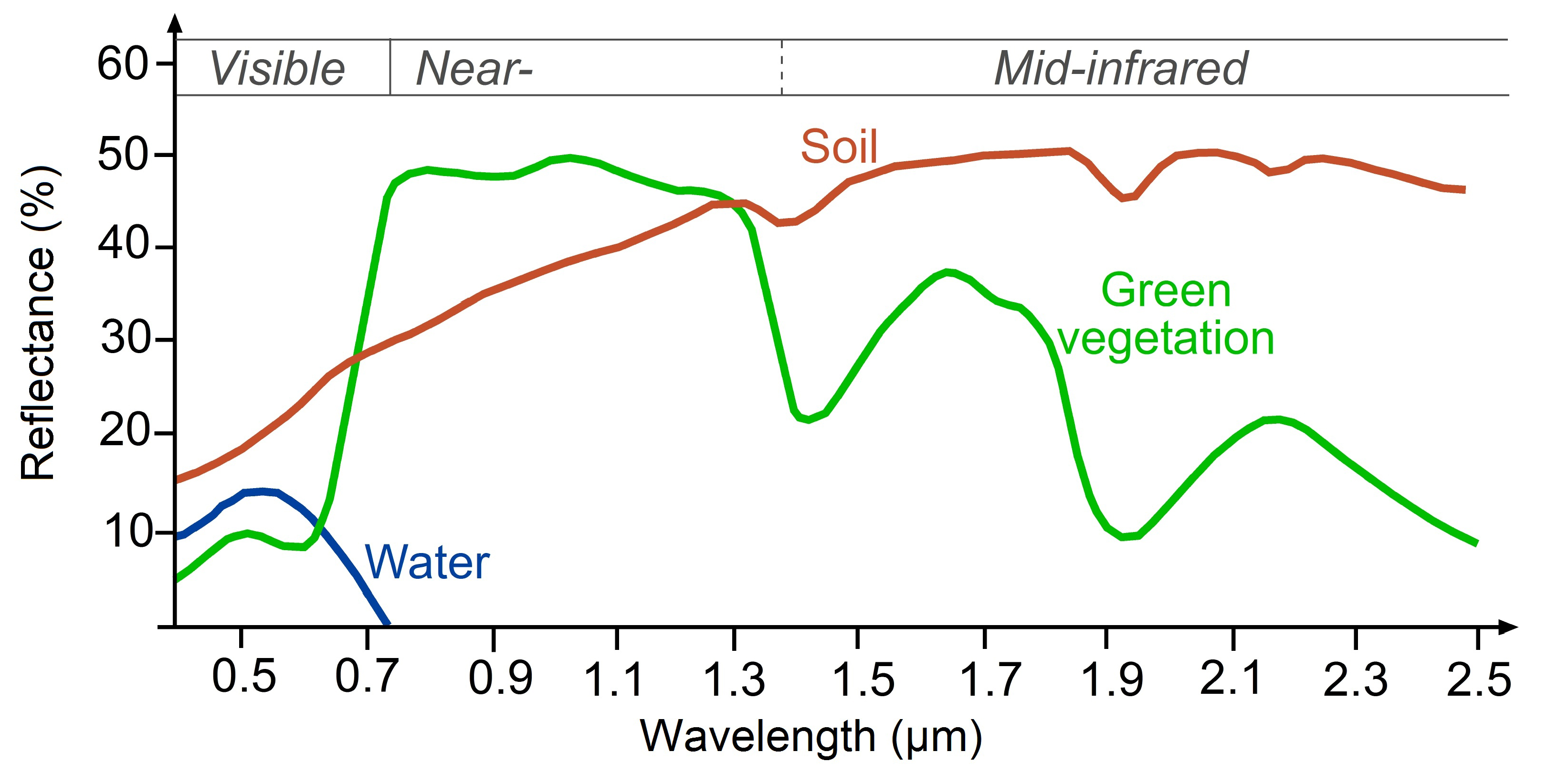
Figure 1.4: Typical spectral signatures of specific land cover types in the visible and infrared region of the electromagnetic spectrum (Source: http://www.seos-project.eu/)
The spectral signature of healthy green vegetation has a small reflectance in the visible portion of the electromagnetic spectrum resulting from the pigments in plant leaves. Most of the light is being used in the photosynthesis process. However, the reflectance increases dramatically in the near infrared. The spectral signature of soil is much less variable. Its behavior is affected by soil moisture, texture, surface roughness and they are less dominant than the absorbance features present in vegetation. The water's spectral signature is characterized by a high absorption at near infrared wavelengths range and beyond. Because of this absorption property, water bodies as well as features containing water can easily be detected, located and delineated with remote sensing data.
These differences make it possible to identify different Earth surface features or materials by analysing their spectral reflectance patterns or spectral signatures. [add more text]
References
Fischer, W. A., W.R. Hemphill and A. Kover. 1976. Progress in Remote Sensing. Photogrametria, Vol. 32, pp. 33-72
Lintz, J. and D. S. Simonett. 1976. Remote Sensing of Environment. Reading, MA: Addison-Wesley. 694 pp.
Barrett, E. C. and C. F. Curtis. 1976. Introduction to Environmental Remote Sensing. New York: Macmillian, 472 pp.
Colwell, R. N. 1966. Uses and Limitations of Multispectral Remote Sensing. In Proceedings of the Fourth Symposium on Remote Sensing of Environment. Ann Arbor: Institute of Science and Technology, University of Michigan, pp. 71-100.
1.1.2 Google Earth Engine's Application Programming Interface (API) and Java Script
Google Earth Engine is a cloud-based platform for scientific data analysis and remote sensing data processing. It provides a large catalog of ready-to-use, cloud-hosted datasets. One of Earth Engine's key features is the ability to handle computationally demading processing and analysis very fast by distributing them across a large number of servers. The ability to efficiently use the cloud-hosted datasets and computation is enabled by the Earth Engine API.
An API is a way to communicate with Google Earth Engine servers. It allows you to specify what computation or command you would like to do, and then to receive the results back from the servers. The API is designed so that users do not need to worry about how the computation is distributed across a cluster of machines and the results are assembled. Users of the API simply specify what needs to be done. This greatly simplifies the code by hiding the implementation detail from the users. It also makes Earth Engine simpler for users who are not too familiar with writing code.
JavaScript API and Introduction to the Code Editor
The Earth Engine platform comes with a web-based Code Editor that allows you to start using the Earth Engine JavaScript API without any installation. It also provides additional functionality to display your results on a map, save your scripts, access documentation, manage tasks, and more. It has a one-click mechanism to share your code with other users—allowing for easy reproducibility and collaboration. In addition, the JavaScript API comes with a user interface library, which allows you to create charts and web-based applications with little effort.
The Code Editor is an integrated development environment for the Earth Engine JavaScript API. It offers an easy way to type, debug, run, and manage code. Once you have successfully registered for a Google Earth Engine account, you can visit https://code.earthengine.google.com/ to open the Code Editor. When you first visit the Code Editor, you will see a screen such as the one shown below:
Figure 1.5: Earth Engine Code Editor
The Code Editor allows you to type JavaScript code and execute it. When you are first learning a new language and getting used to a new programming environment, it is customary to make a program to display your name or the words “Hello World.” This is a fun way to start coding that shows you how to give input to the program and how to execute it. It also shows where the program displays the output. Doing this in JavaScript is quite simple. Copy the following code into the center panel:
print('Hello World');The line of code above uses the JavaScript print() function to print the text “Hello World” to the screen. Once you enter the code, click the Run button. The output will be displayed on the upper right-hand panel under the Console tab:
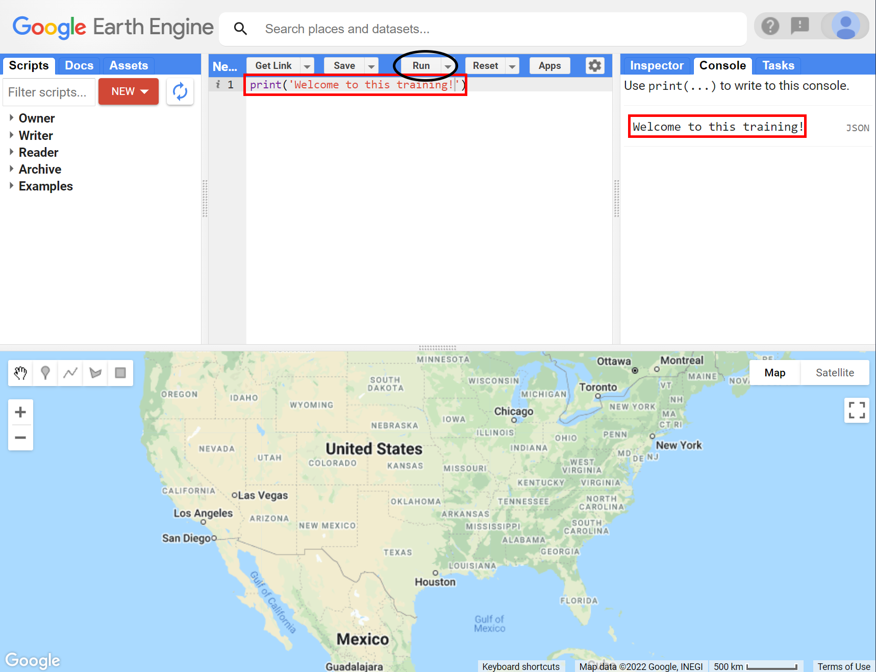
Figure 1.6: Running code with GEE
You now know where to type your code, how to run it, and where to look for the output. You just wrote your first Earth Engine script and may want to save it. Click the Save button to save a script:
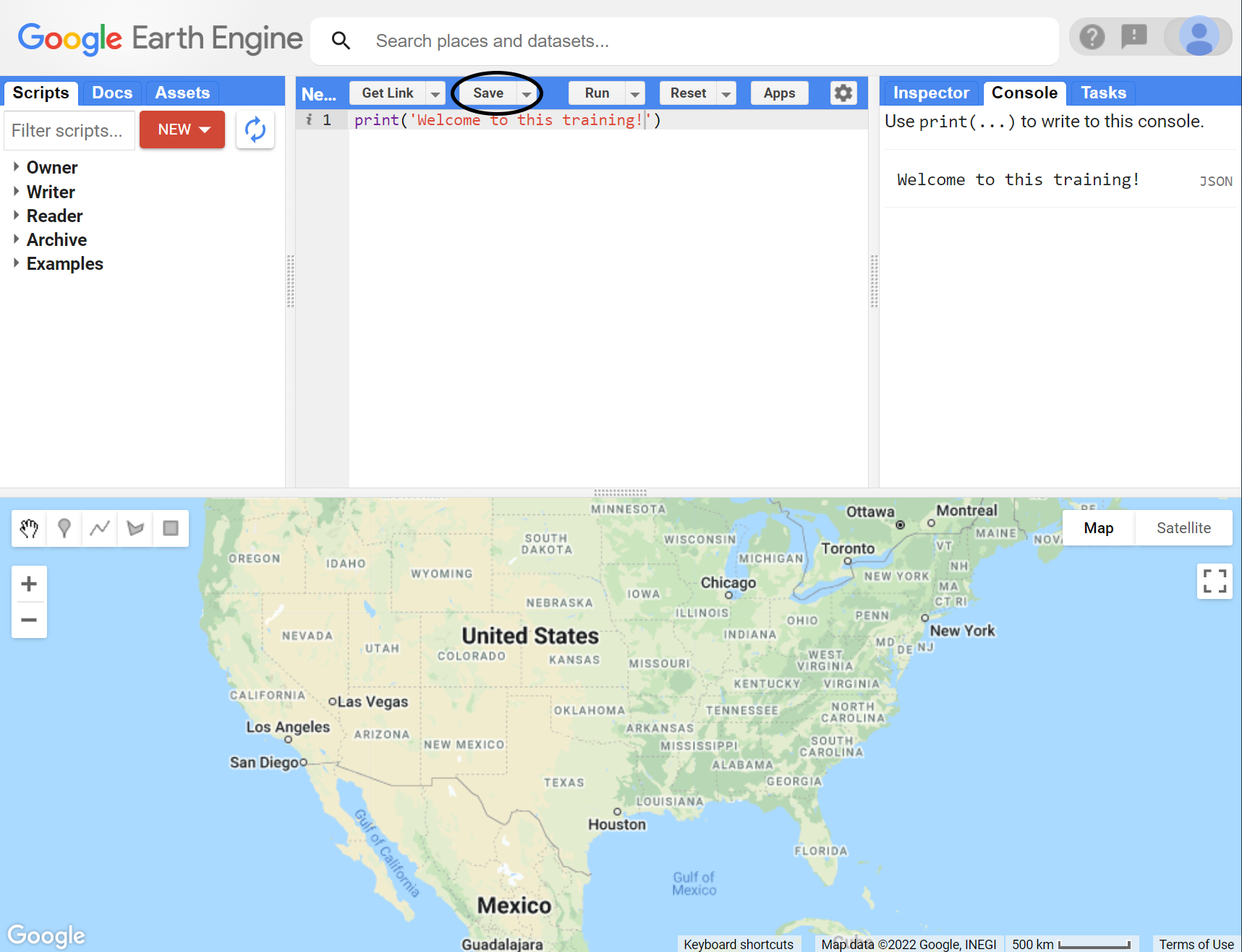
Figure 1.7: Saving a script
If this is your first time using the Code Editor, you will be prompted to create a home folder. This is a folder in the cloud where all your code will be saved:
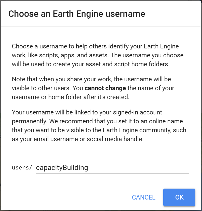
Figure 1.8: Your first home folder
You can pick a name of your choice, but remember that it cannot be changed and will permanently be associated with your account.
Once youre home folder is created, you will be prompted to create a new repository. A repository is a like a folder where you can save your scripts. You can also share entire repositories with other users. Your account can have multiple repositories and each one can hold multiple code scripts. Start by creating a repository:
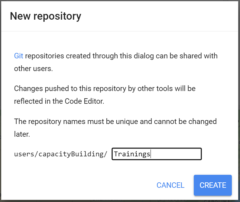
Figure 1.9: Your first repository
Finally, you will be able to save your script inside the newly created repository. Enter a name of your choice and click OK:
Spaces are not allowed when naming scripts!
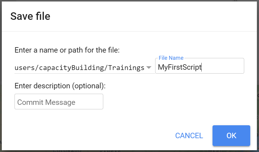
Figure 1.10: Saving a script file
Once the script is saved, it will appear in the script manager panel. The scripts are saved in the cloud and will always be available to you when you open the Code Editor.
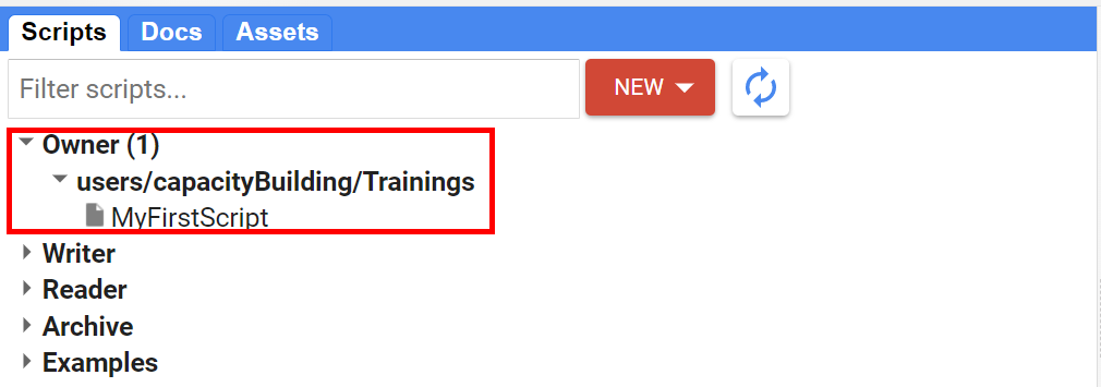
Figure 1.11: Your first script in your repository
JavaScript Basics: Data types
Javascript is the language you will use to construct and set up your commands and analysis. This section covers the basics of the Java Script sintax and some basic data structures. In the following sections, more JavaScript code will be presented. Throughout this document, code will be presented with a distinct colored font and with shaded background. As you encounter code, copy and paste it into the Code Editor and click Run.
A) Variables
In a programming language, variables are used to store data values. In JavaScript, a variable is defined using the var keyword followed by the name of the variable. For instance, create a var named city that contain the text string 'Monrovia'. Text strings in the code must be always in quotes. Google Earth Engine allows you to use single ' or double " quotes, as long as they match in the beginning and end of the text string. We also usually end each statement on scripts with a semicolon ;, although Earth Engine's code editor does not require it. A 'i' will be shown in the line of the code where a semicolon is missing:

Figure 1.12: Even though they are not a requirement, Google Earth Engine indicates that a semicolon is missing in the statement. You can hover the mouse cursor over the icon to reveal its meaning.
var city = 'Monrovia';If you print the variable city, you will get the string stored in the variable (Monrovia) printed in the Console.
print(city);When you use quotations, the variable is automatically assigned the type string. You can also assign numbers to variables. For example, create the variables population and area and assing a number as their value. When assigning numbers, you do not use commas , for thousand separators. You do, however, use . for decimals:
var population = 939524;
var area = 194.25;
Print those variables to the Console. You can also add text to describe the variables printed in the Console. Simply add a text string within the print function along with the variable being printed separated with ,. Use the code below as example:
print('Number of people in Monrovia:', population);
print(area, 'km squared');
B) Lists
In the previous examples, we created variables holding a single value (text or number). JavaScript provides a data structure called a list that can be used When you want to store multiple values in a single variable. You can create lists using square brackets [] and adding multiple values separated by ,. Create a variable called listofcities, add values to it and print it to the Console:
var listofcities = ['Monrovia', 'Gbarnga','Kakata', 'Bensonville'];
print('Largest cities in Liberia', listofcities);
Looking at the output in the Console, you will see listofcities with an expander arrow (▹) next to it. Expand the list by clicking on the arrow to show its content. You will notice that along with the items on the list, there will be a number next to each value you added. This is the index of each item. It allows you to refer to each item in the list using a numeric value that indicates its position in the list. This is useful when you want to extract a particular item from a list object.
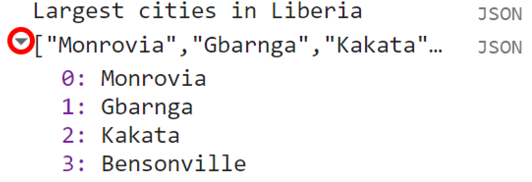
Figure 1.13: A JavaScript List.
C) Objects and Dictionaries
While useful to hold multiple values, lists are not appropriate to hold more structured data. JavaScript allows you to store 'key-value' information in objects or dictionaries. In this type of data structure, you can refer to a value by its key rather than its position - like in lists. You can create objects using curly braces {}. Use the code below as an example of an object:
var cityData = {'city': 'Monrovia', 'population': 939524, 'area': 194.25, 'coordinates': [-10.790, 6.315]};There are a few important things about the syntax of the code above: As objects tend to hold several keys and values, it can be difficult to read the code if it is written on a continuous string. To improve readability you can use multiple lines instead:
var cityData = {
  'city': 'Monrovia',
  'population': 939524,
  'area': 194.25,
  'coordinates': [-10.790, 6.315]
};
Note how each key-value pair is on a different line. It is much easier to organize your key-value information this way. Additionally, the code can be more easily read. Second, note that the object above can holds multiple types of types of values (string and numbers) and structure (list)!
If you print cityData to the Console, you can see that instead of a numeric index, each value will be identified by its key.
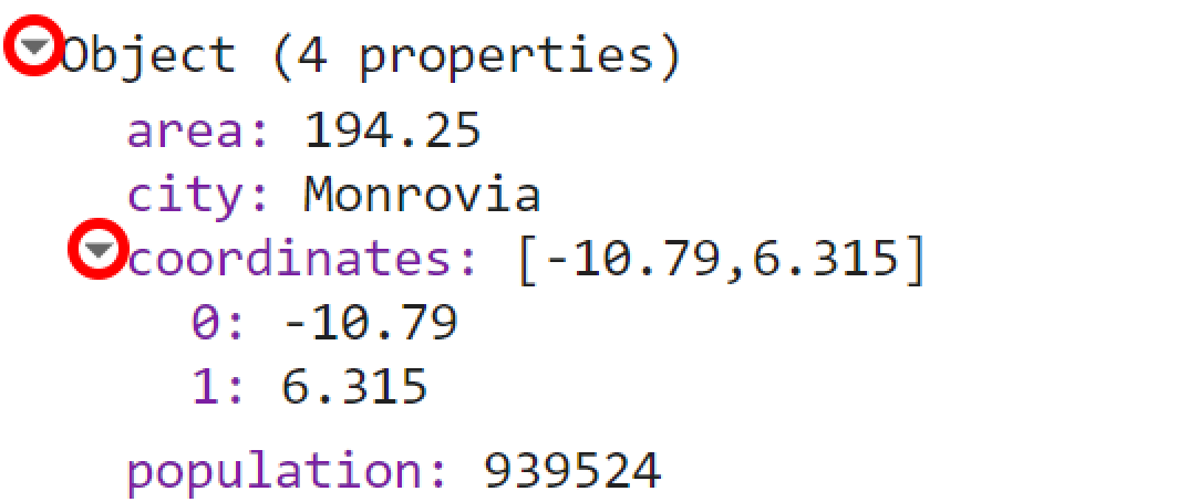
Figure 1.14: A JavaScript Object.
This key can also be used to retrieve the value of an item within an object or dictionary. If you want to retrieve a particular key from a dictionary, simply use ['key']. For example, if you want to retrieve the population value from this object and print it individually to the Console, you can use a code like this:
print(cityData['population']);The same logic can be applied to lists. Always remember that lists have numeric index. Therefore, when retrieving itens from a list, use the number of its position on the list:
print(listofcities['2']);D) Functions
Functions are often used to group a set of operations and used to repeat the same operation with different set of parameters without having to rewrite the code for every iteration. In other words, you can call a function with different parameters to generate different outputs without changing the code. Functions are defined using function(). They often take parameters which tell the function what to do. These parameters go inside the parentheses (). Below is an example of a function named SumFunction to calculate the sum of two numbers: fistValue and secondValue. The var sum adds those two parameters and return is used to generate the output of that operation
function SumFunction (firstValue, secondValue) {
  var sum = firstValue + secondValue;
  return sum;
}
Note that if you run the code above, nothing happens. This is just a function and it needs to be given the parameters. For example, if you need to add 37 to 584 using this function and print the result into the Console, you can use the code below:
var result = SumFunction(37,584);
print(result);
When you call SumFunction, it will always perform the operation sum with watever two parameters you define in (). As mentioned, you can perform several operations at once using functions. For example, you can add other operations in the function above and return a list or a dictionary with the results:
function MathFunction (firstValue, secondValue) {
  var sum = firstValue + secondValue;
  var sub = firstValue - secondValue;
  var fraction = firstValue / secondValue;
  return {'Result Sum':sum, 'Result Substraction':sub, 'Result Division': fraction};
}
Using MathFunction with a pair of parameters (firstValue and SecondValue) will return an object with the results of each operation:
var results = MathFunction(500,5);
print(results);
Figure 1.15: Printed results of MathFunction.
Earth Engine Containers and Objects
So far, you learned the different data structure/types you can use within Google Earth Engine. However, if you want to do any computation with the data stored in these different types of structure, you will have to use an Earth Engine container. The ee package is used for formulating requests to Earth Engine. In other words, ee (prefix for Earth Engine) allows you to request Earth Engine servers to perform a certain computation to an variable or object. Each ee object has many different methods. You can think of methods as the many different things and computations that can be done for an specific object. In the Code Editor, you can switch to the Docs tab to see the API functions grouped by object types.
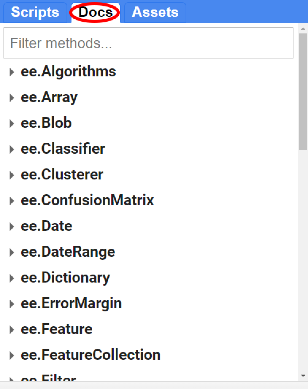
Figure 1.16: List of available objects in the Docs tab of GEE API.
Below are some examples to ilustrate the concept behind an Earth Engine object:
A) Strings
You can put strings into a ee.String object to be sent to Earth Engine. Using an object/container allows you to do manipulate them in many different ways. For example, ee.String has the: * toLowerCase() method. This method will convert any string in a ee.String object to lower case; * length() method. This method will count the characters in your string; * cat() method. This method will concatenate two strings into one; * and many others! Make sure to check the Docs tab for all the available methods for a given object.
The code below uses some of the methods of ee.String as an example:
var string = ee.String('HELLO EVERYONE, ');
print(string.toLowerCase());
print(string.length());
var string2 = ee.String('nice to meet you');
print(string.cat(string2));
In your console tab you will see that the 'HELLO EVERYONE, ' string is now all in lower case. You will also see that .length() returned 16 as the number of characters for that string.
Consider the code below:
var string = 'HELLO EVERYONE';
var string2 = 'nice to meet you';
print(string.cat(string2));
If you try to use a method on a non ee object, you will get an error.
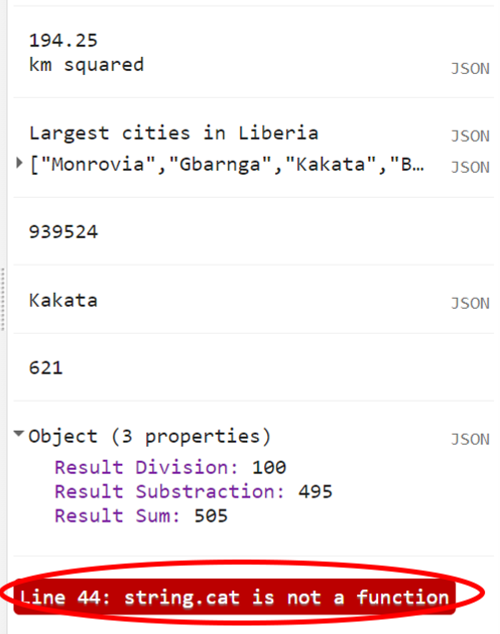
Figure 1.17: Trying to use a method on non-ee.Object will return an error
B) Numbers
ee.Number is just another example of an object from that list. Similarly to ee.String, it will have many methods to be used with. For example, .add(), .subtract(), .divide() and .multiply () will perform these operations on ee.Number objects. Make sure to consult the Docs tab for all the different methods for each object.
var value1 = ee.Number(100);
var value2 = ee.Number(2);
print(value1.add(value2));
print(value1.subtract(value2));
print(value1.divide(value2));
print(value1.multiply(value2));
print(value1.log10());
B) Lists
You can also make a JavaScript list into an ee.List on Earth Engine server by simply casting your list into the container. There are many other useful methods to use when you have an ee.List. For instance, instead of making a JavaScript list by typing each value, you can use ee.List.sequence() to construct a list. This method will take many arguments, such as the value of the start of the list, the value at the end of the list, steps (increment) and count. Consider the examples below:
- Making a list with numbers from 0 to 10:
print('List 1', ee.List.sequence(0,10))- Making a list from 0 to 10 with increments of 2:
print('List 2', ee.List.sequence(0,10,2))
Remember: A var string = 'text' is a JavaScript string that does not allow computations. A var string = ee.String('text') is an Earth Engine object that allows computations!
1.1.3 Exploring Image and Image Collection
Now that you learned the basics of JavaScript and Earth Engine objects, you have the tools at your disposal to start using the Earth Engine API to build scripts for remote sensing analysis. In this section, we explore satellite imagery, which are one of GEE's core capabilities!
A) Single band image
The first thing you need to know is that when working with images in Earth Engine, you will have to use an ee.Image() container. The argument provided to the constructor is the string ID of an image in the Earth Engine data catalog. (Remember to always see the Docs tab for a full list of arguments to this container). To retrieve an image ID, you can search in the Earth Engine catalog using the search tool at the top of the Code Editor:
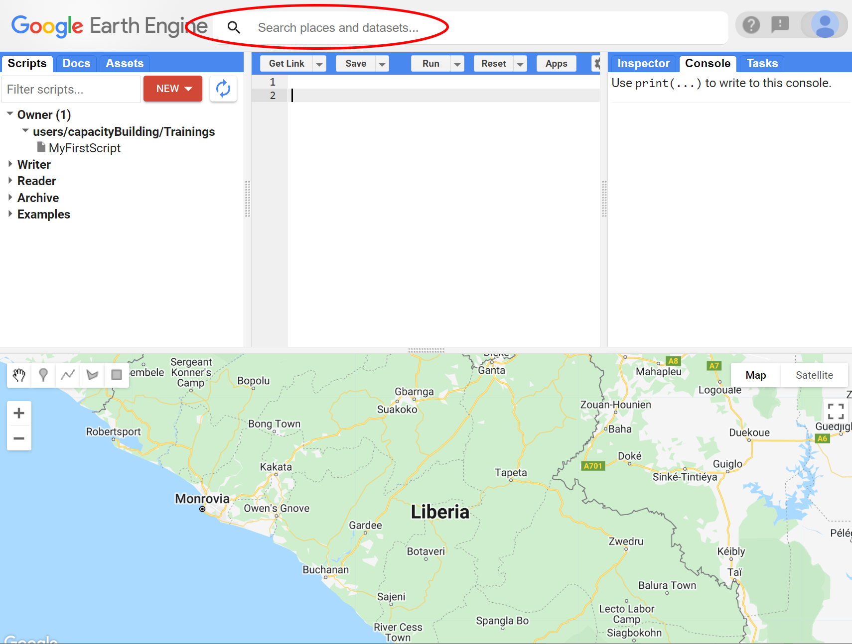
Figure 1.18: You can browse through Earth Engine's data catalog with the search tool
For example, try typing 'elevation' into the search field and note that a list of rasters is returned:
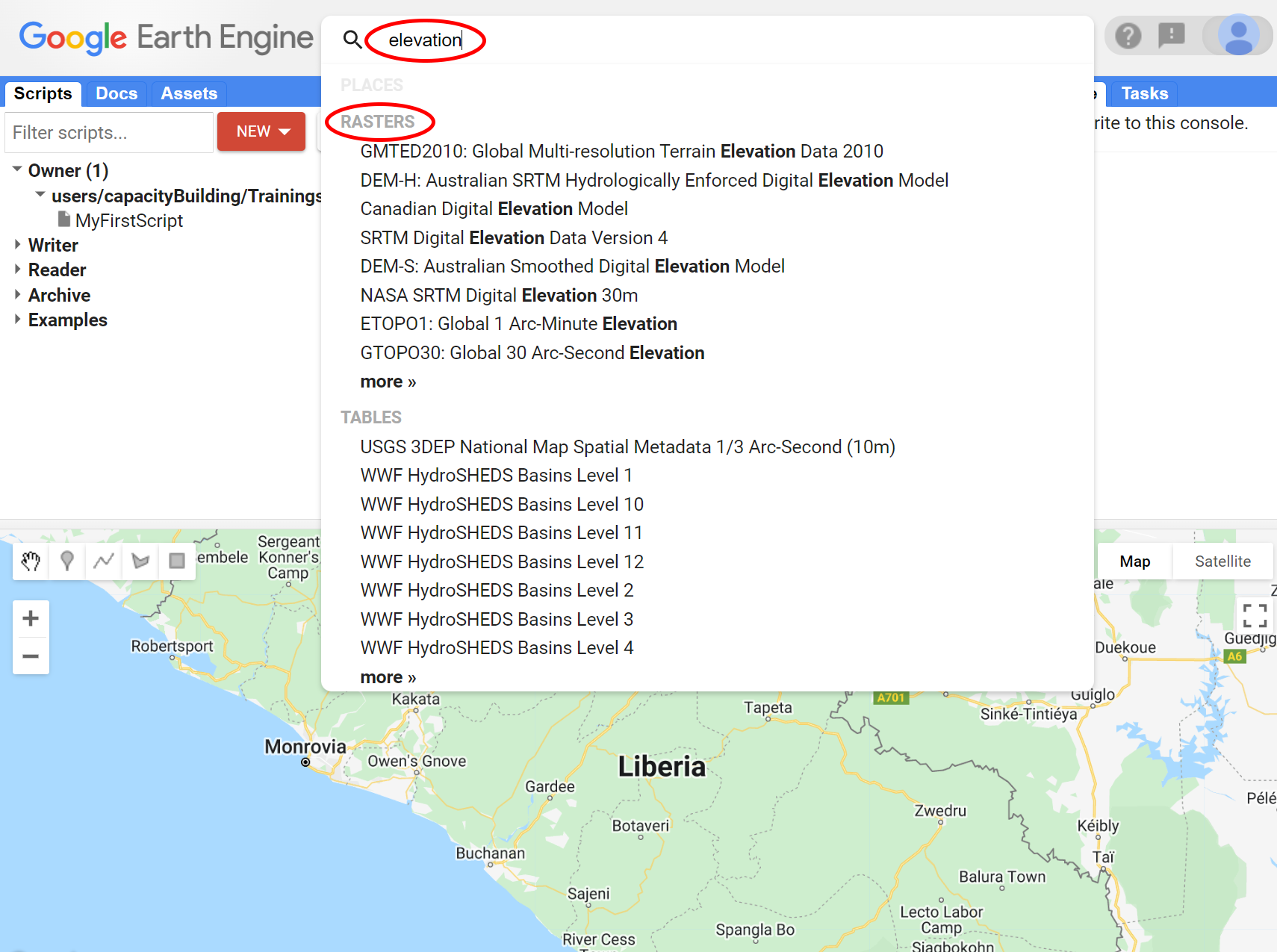
Figure 1.19: Typing in the search field. Google Earth Engine will show all datasets available with that criteria.
Click in any of the dataset entries to see more information about that dataset. From the list above, explore the dataset 'SRTM Digital Elevation Data Version 4'. You can also find more information about this dataset on the tabs on the top right side of the dataset description screen. On the left side of the dataset description screen, you can find the Image ID, which is what we use with the ee.Image(). Alternatively, you can use the Import button on the dataset description. Using the Import button, a variable is automatically created in a special section, named 'Imports', at the top of your script. You can rename the variable by clicking on its name in the imports section.
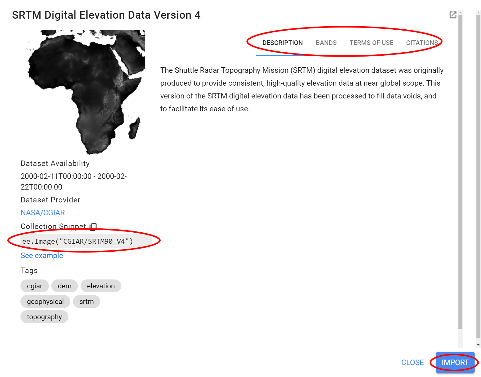
Figure 1.20: Data description
Copy the image ID from the screen above and add it to a var elevationImage with the ee.Image() container as shown below:
var elevationImage = ee.Image('CGIAR/SRTM90_V4');You can also retrieve the metadata about this image by using print(). In the Console, click the expander arrows to show the information. You will discover that the SRTM image has one band called 'elevation'.
print(elevationImage);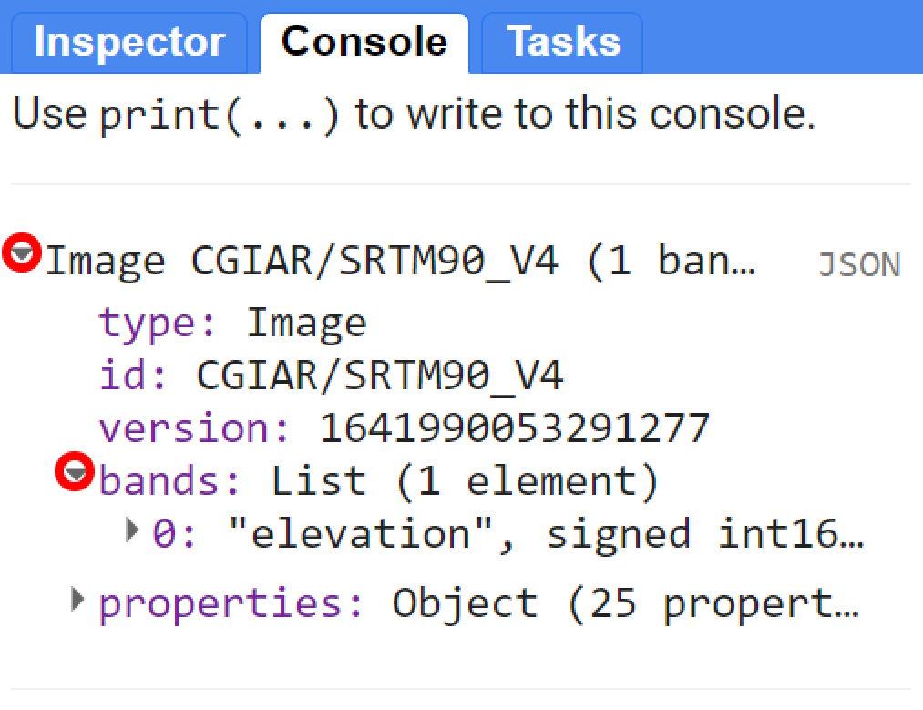
Figure 1.21: Image description using print()
To display the image in the Map Editor, use the Map object's .addLayer() method. When you add an image to a map using Map.addLayer(), Earth Engine needs to determine how to map the values in the image band(s) to colors on the display. If a single-band image is added to a map - which is our case- by default Earth Engine displays the band in grayscale, where the minimum value is assigned to black, and the maximum value is assigned to white. If you don't specify what the minimum and maximum should be, Earth Engine will use default values.
Map.addLayer(elevationImage);Do not worry! You can make it look better with custom visualization parameters!
To change the way the data are stretched, you can provide another parameter to the Map.addLayer() call. Specifically, the second parameter, visParams, lets you specify the minimum and maximum values to display. One way of gauging the range of values of an image is by activating the Inspector tab and click around on the map. You will be able to see the value of that band for this dataset at that particular location:
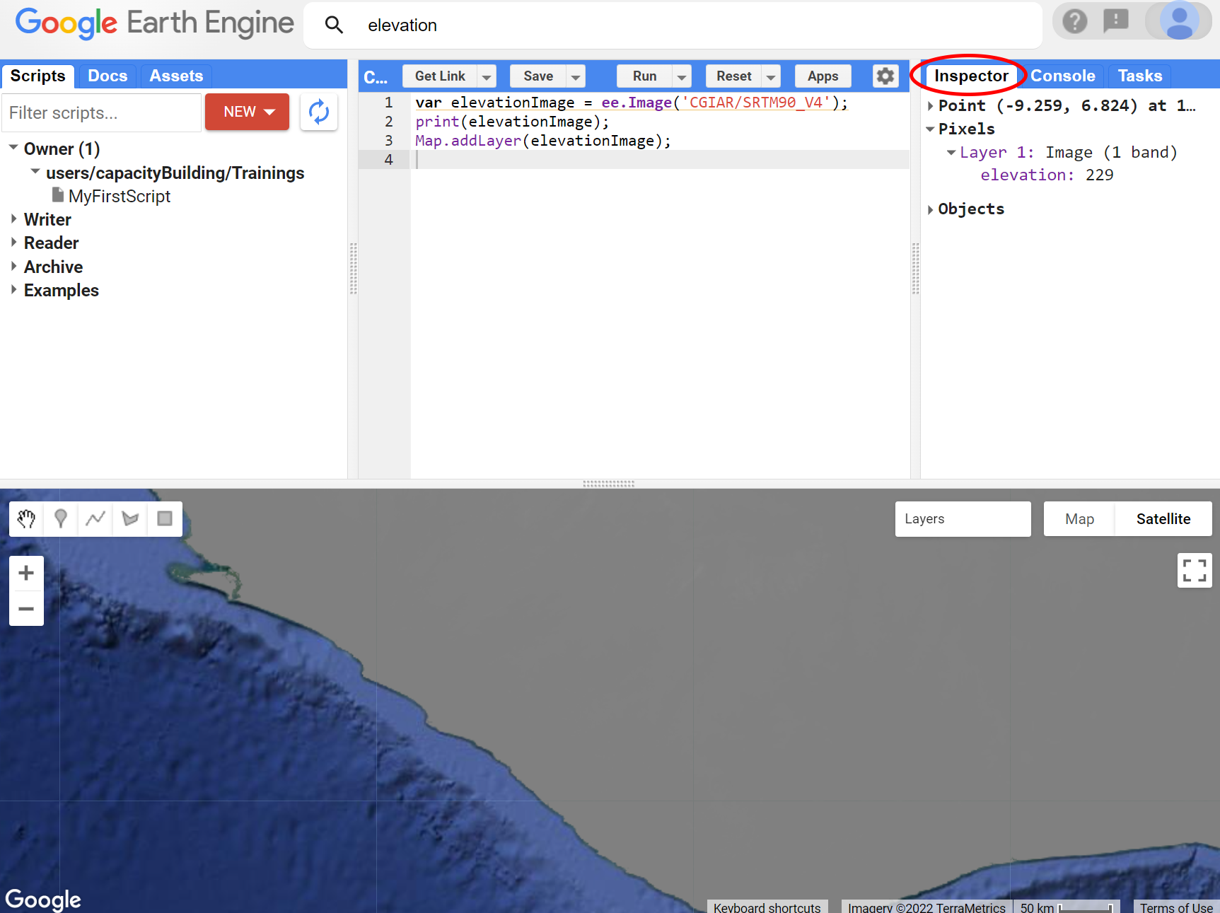
Figure 1.22: Inspector tab. Click in the image and the inspector tab will display the data for that point
Click around the area of Liberia to have a sense of the range of values for this dataset. Suppose that, through further investigation, you determine that the best range of values to display elevation data in Liberia is [0,1000]. To display the data using this range, you can use a dictionary containing two keys: min and max and their respective values 0 and 1000. A third parameter for Map.addLayer() is the name of the layer that is displayed in the Layer manager. Thus your code should be looking like the one below:
Map.addLayer(elevationImage, {min:0, max:1000}, 'Custom Visualization');Run the code and you will see something like:
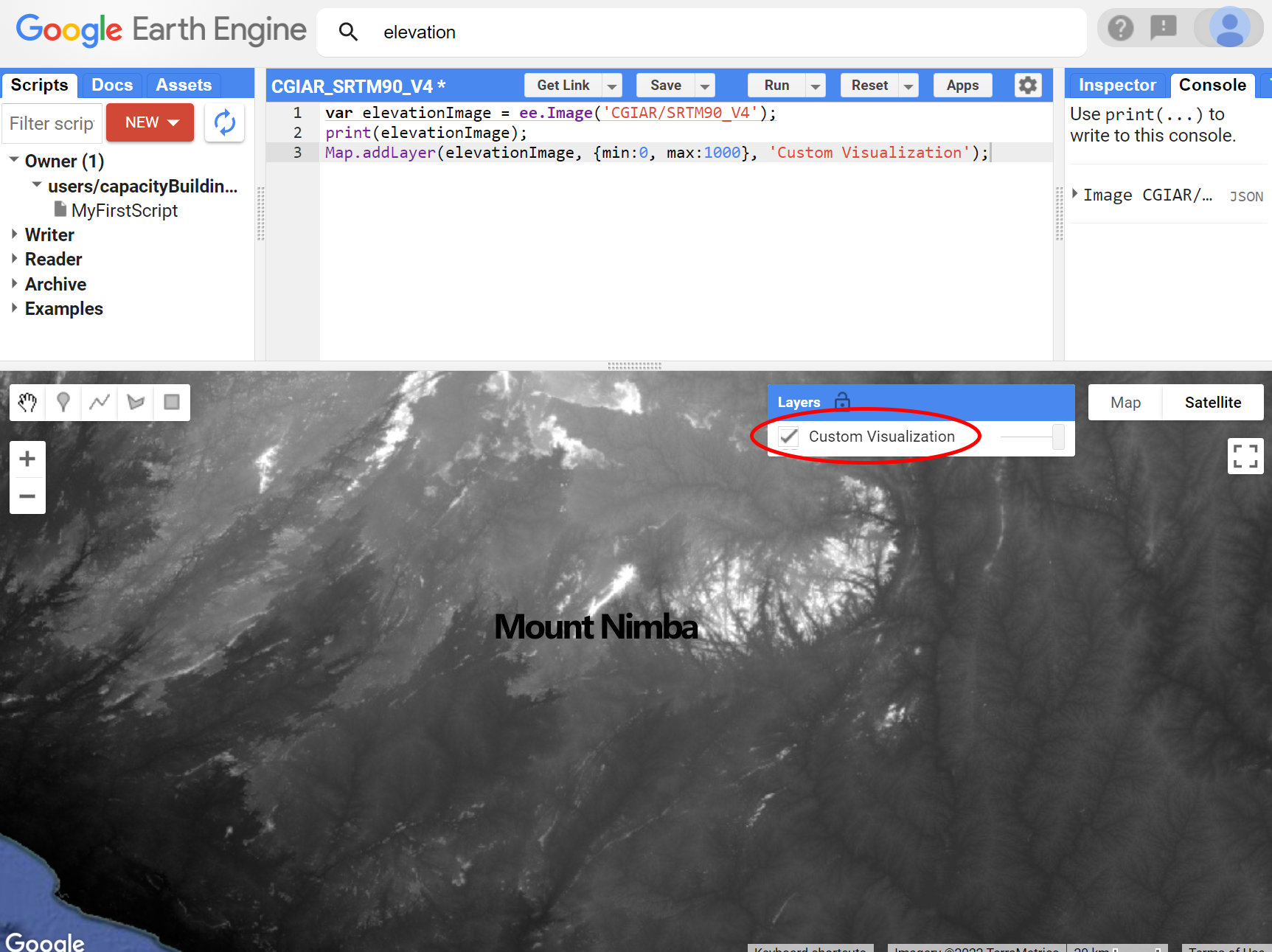
Figure 1.23: Custom Visualization for the SRTM data based on range of values.
You can further improve your image display by using a color palette. Palettes let you set the color scheme for single-band images. A palette is a comma delimited list of color strings which are linearly interpolated between the maximum and minimum values in the visualization parameters.
To display this elevation band using a color palette, add a palette property to the visParams dictionary:
Map.addLayer(elevationImage, {min:0, max:1000,palette: ['green', 'yellow', 'red']}, 'Custom Visualization - Color');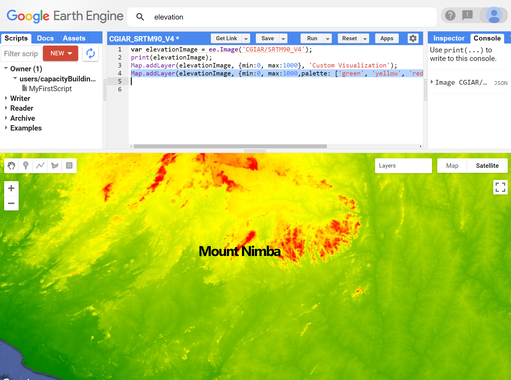
Figure 1.24: Custom Visualization for the SRTM data based on range of values and color palette.
In the next section, you'll learn how to display multi-band imagery.
B) Multi band image
To ilustrate the concepts and codes in this section, we will use a Landsat 8 image from April 2022 over Cairo, Egypt. Landsat is a set of multispectral satellites developed by the NASA (National Aeronautics and Space Administration of USA), since the early 1970’s. Landsat images are very used for environmental research. These images have from 8 to 11 spectral bands (spectral resolution), with pixels of 30x30 meters (spatial resolution) and with a revisit time of 16 days (temporal resolution).
Copy and paste the code below into the Code Editor:
var ImageL8 = ee.Image('LANDSAT/LC08/C02/T1_L2/LC08_176039_20220406');As learned before, the code above is casting a Landsat 8 image into an ee.Image container using its ID into a var called 'ImageL8'. By clicking Run, Earth Engine will retrieve this image from its Landsat image catalog. You will not yet see any output.
As you learned, you can retrieve additional information about this image by using print().
print(ImageL8)In the Console panel, you may need to click the expander arrows to show the information. You should be able to read that this image consists of 19 different bands (index 0 to 18). Each band will have 4 properties: name, data type (as in if the value is an integer, float, ect.), projection and dimensions (in rows and columns of pixels). For this example, simply note the first property of the first band:
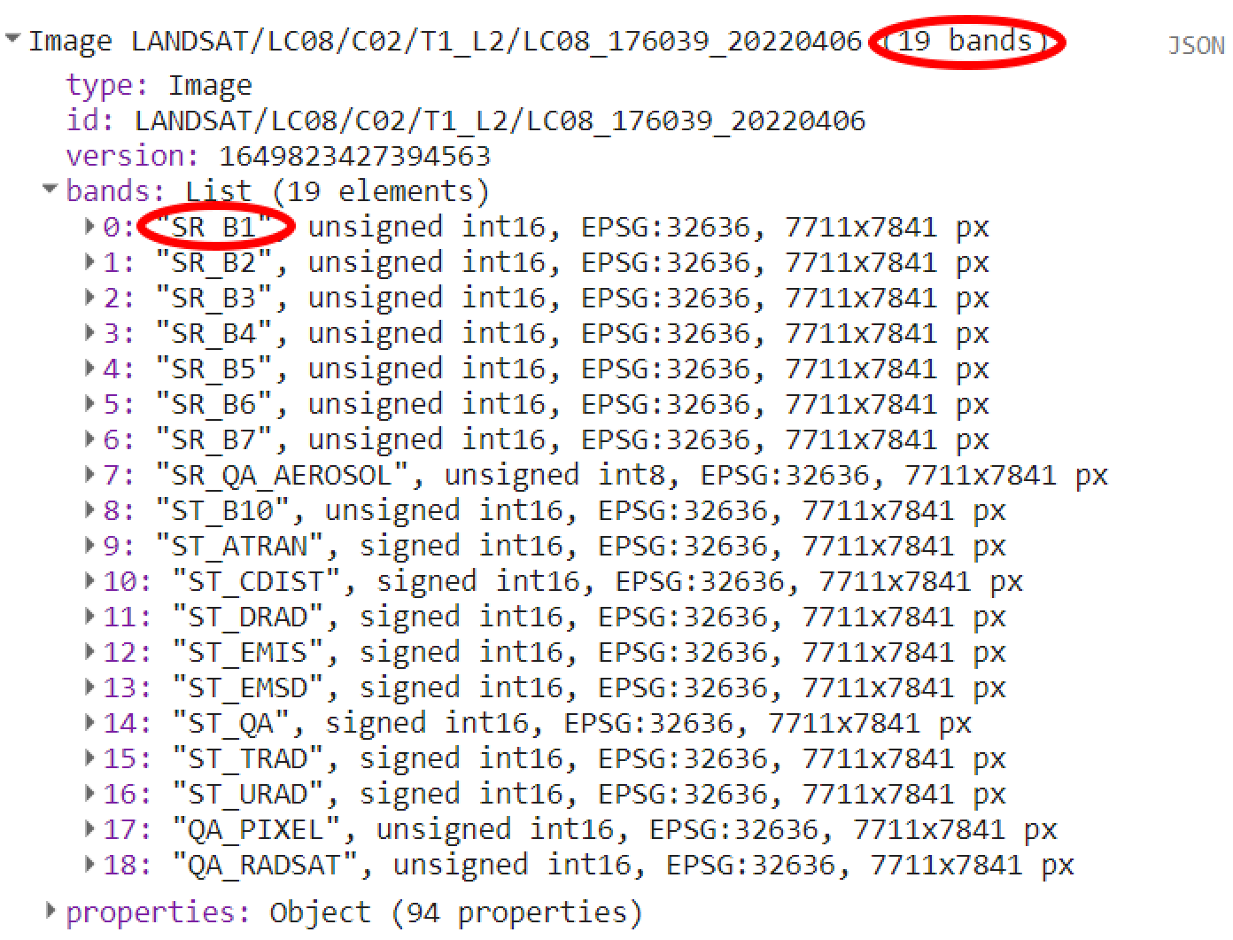
Figure 1.25: Landsat 8 image metadata.
A satellite sensor like Landsat 8 measures the EMR in different portions of the electromagnetic spectrum. Six out of seven first bands in our image ("SR_B2" through "SR_B7") contain measurements for six different portions of the spectrum:
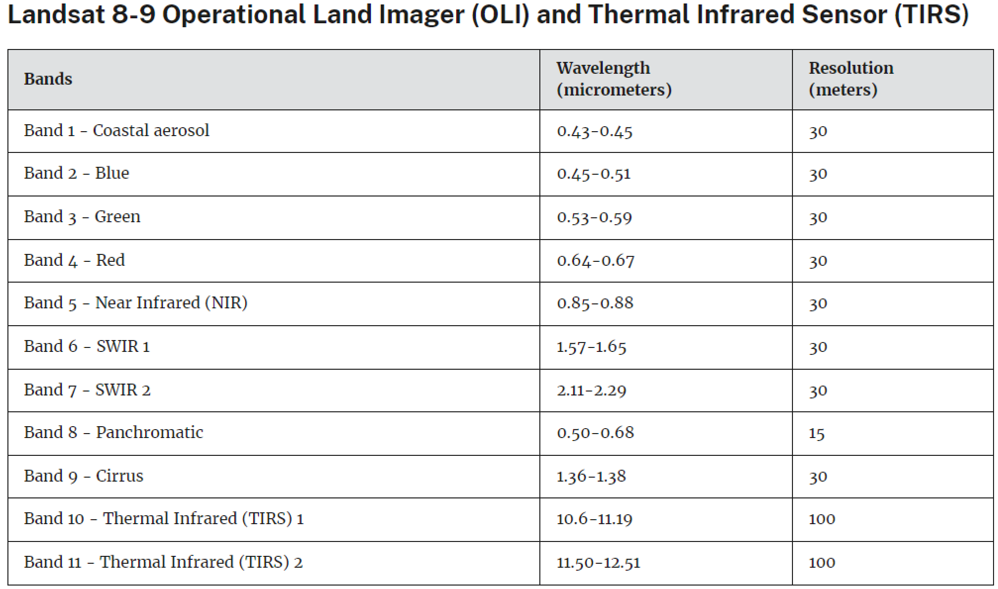
Figure 1.26: Landsat 8 bands. Source: https://www.usgs.gov/faqs/what-are-band-designations-landsat-satellites
Now, let's visualize ImageL8. First, make sure your map is somewhere near Cairo, Egypt. To do this, click and drag the map towards Cairo, Egypt. (You can also jump there by typing “Cairo” into the Search panel at the top of the Code Editor). Add ImageL8 to the Map as a layer using the code below:
Map.addLayer(ImageL8);You probably see a gray image with not a lot of details. From the previous section you learned that Map.addLayer take many parameters. One of them is the visParams, which lets you specify the minimum and maximum values to display. Similarly to the previous section, you can use the Inspector tab to investigate the range of values for each location for each of ImageL8's band. Now, specify a range of values to be displayed. Follow the code example below:
Map.addLayer(ImageL8, {min:8000, max:20000}, 'My First Image');You should see something like this:
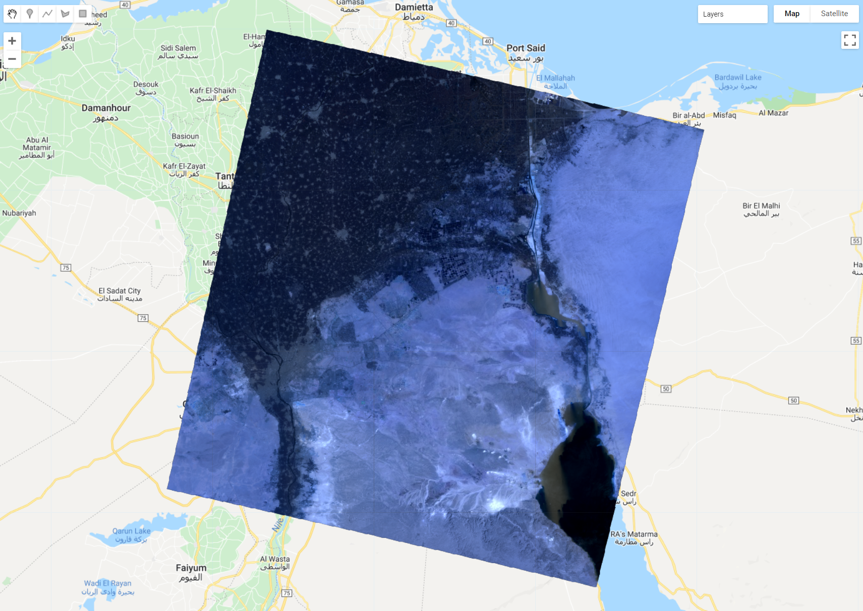
Figure 1.27: Landsat 8 image in false color .
By default, if you do not specify the bands to be displayed within the visParams, Earth Engine will display the first three bands, each band on each RGB (red, green, blue) channel of your monitor screen. In other words, Earth Engine is displaying 'SR_B1' (Landsat 8's coastal aerosol band) in the red channel, 'SR_B2' (Landsat 8's blue band) in the green channel and 'SR_B3 (Landsat 8's green band). This is a case of a false color display, when spectral bands do not match the RGB channels in your screen. False color displays have many advantages and they will be explored later in the tutorial.
For a real color display, you will need to define the bands within visParams to match the RGB channels:
Map.addLayer(ImageL8, {bands: ['SR_B4', 'SR_B3', 'SR_B2'], min:8000, max:20000}, 'Real color');In the code above, visParams contains a list (bands) with the names of the ImageL8's bands to be displayed in the RGB channels of your screen. This band set up tells Earth Engine to display the red band in the red channel, the green band in the green channel and the blue band in blue channel. We call this composition a RGB 432 or Real color composition. You should see an image like this when running the code above:
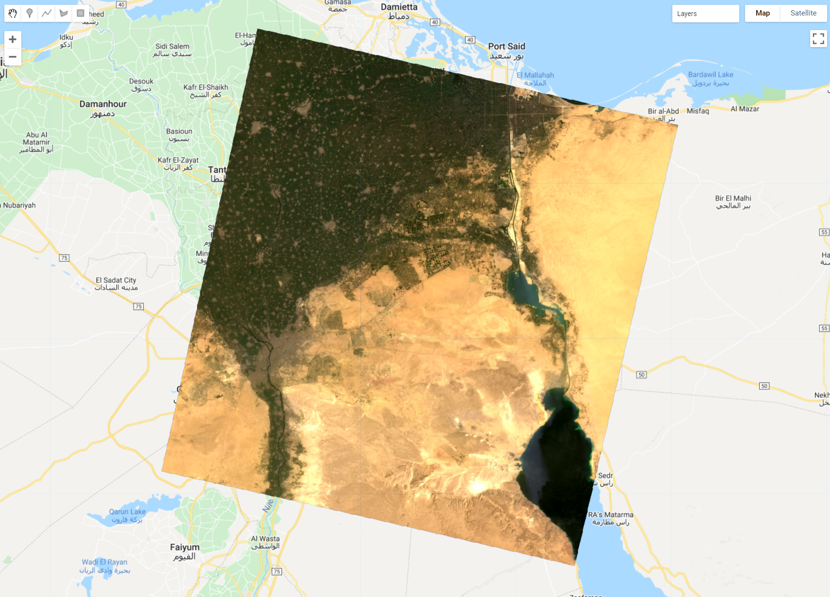
Figure 1.28: Landsat 8 image displayed with a real color composition.
You can easily change these values and settings within visParams by using the Layer setting option in the Map editor. You can find it by hovering your cursor over the Layer List (upper right corner of the Map editor, next to the Map and Satellite buttons) and clicking the gear icon of the layer:
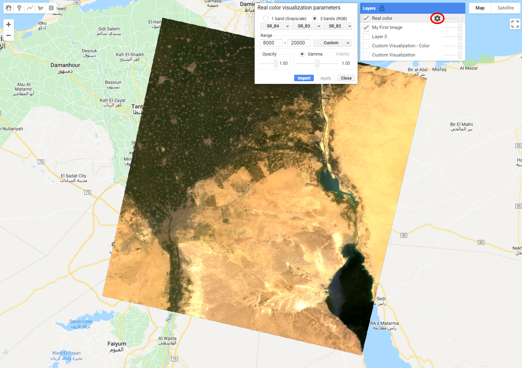
Figure 1.29: Layer settings window.
Once you chose your settings, click Apply. Earth Engine will automatically apply the new settings and display the layer. Try using different band combinations and range values to see how the image changes. Different color compositions will highlight different features in the image based on their spectral signatures!
C) Image collections
An image collection refers to a set of Earth Engine images. For example, the collection of all Landsat 8 images! In this case, you will use ee.ImageCollection() instead of ee.Image() to retrieve a particular image collection . Like the SRTM image or the Landsat image you have been working with, image collections also have an ID. Similarly to the single images, you can discover the ID of an image collection by searching the Earth Engine data catalog from the Code Editor.
Start by loading the Landsat 8 image collection into a var called 'collection using the ee.ImageCollection container. Then try to print this collection to the Console:
var collection = ee.ImageCollection('LANDSAT/LC08/C02/T1_L2');
print(collection);
You will notice that you will get an error when trying to print collection to the Console:

Figure 1.30: Trying to print an image collection without any filter.
It's worth noting that this collection represents every Landsat 8 scene collected, all over the Earth. Thus, Earth Engine is not able to print the information for every scene all over the globe since 2013 (when Landsat 8 started collecting data). In this case we need to filter this collection. Exploring the Docs tab of the Code Editor to learn more about ee.ImageCollection, you will notice the methods filterBounds() and filterDate(). These are shortcut methods on a bigger filter() method. In this case, filterBounds() filters a collection by intersection with geometry (or a location) while filterDate() filters a collection by a date range, expressed as strings.
Location Filter: To filter collection to images that cover a particular location, first define your area of interest with the geometry drawing tools. To create geometries, use the geometry drawing tools in the upper left corner of the map display.
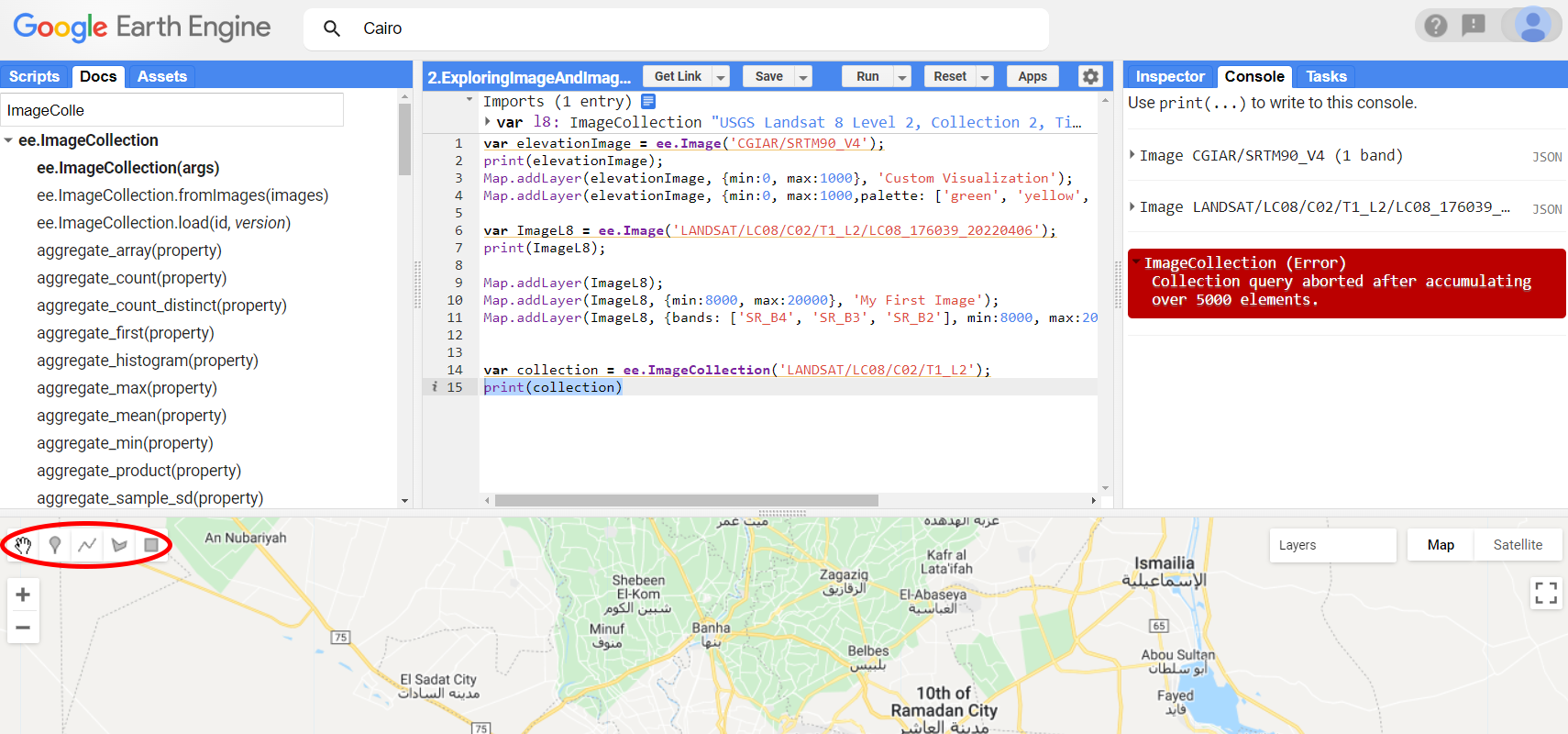
Figure 1.31: The Geometry tools.
For drawing points, use the place mark icon, for drawing lines, use the line icon, for drawing polygons, use the polygon icon, for drawing rectangles, use the rectangle icon. Using any of the drawing tools will automatically create a new geometry layer and add an import for that layer to the Imports section (top of the script). Once you finish drawing the geometry, click Exit. To rename the geometries that are imported to your script, click the settings icon next to it (or rename it directly in the Imports section).The geometry layer settings tool will be displayed in a dialog where you can change the geometry name.
Use the point mark and create a point geometry named 'aoi' (area of interest) in a location of your interest. For this example, we will use a point mark location over Cairo, Egypt. Use the figure below as a guide: 1) Click on the point mark geometry; 2) Place it in your location of interest, and; 3) rename it 'aoi'.
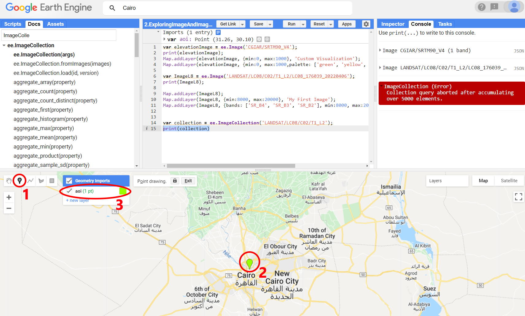
Figure 1.32: Creating a point geometry.
Date filter: Now that you have a location, create two variables startDate and endDate containing a data range expressed as strings. Use a date range of your choice. Dates are expressed as 'YYYY-MM-DD' in Earth Engine. For this example, we will use the first four months of 2022:
var startDate = '2022-01-01';
var endDate = '2022-04-30';
Now that you have both filters for location and date range, you are ready to filter your image collection using filterBounds() and filterDates():
var collectionFiltered = collection.filterBounds(aoi).filterDate(startDate,endDate);
print(collectionFiltered);
When printing collectionFiltered to the Console you will notice that now Earth Engine was able to retrieve the information of every Landsat scene based on your filters. Using the date range and the location filters from this example, there are the 13 images in the collectionFiltered for Cairo from January to April, 2022:
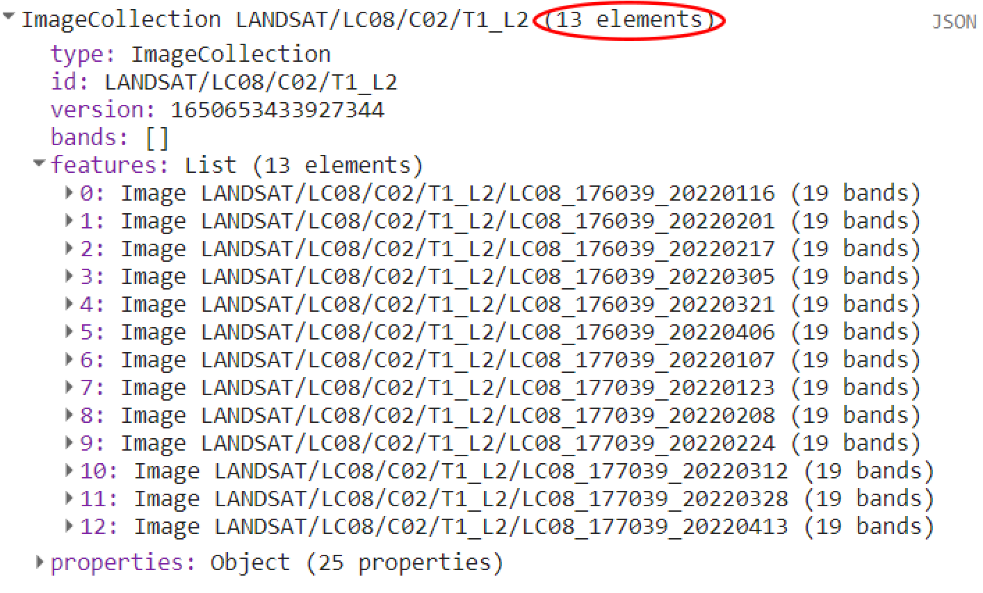
Figure 1.33: Filtered collection.
If you want to retrieve a particular image from this collection you can simply use ee.Image() and the image ID printed in the Console tab!
1.2 Image and Image Collection Manipulation
Now that you know how to load and display an image, it's time to apply a computation to it. In the following sections you will learn some examples of computations for a single-band image and multi-band image (band math and vegetation index calculation) and for an image collection.
1.2.1 Image Math
- Single-band image
Considering our previous example, we will use the SRTM single-band image elevationImage and create a 'slope' image. Briefly, you calculate the slope by dividing the difference between the elevations of two points by the distance between them, then multiply the quotient by 100. The difference in elevation between points is called the rise. The distance between the points is called the run. Thus, percent slope equals (rise / run) x 100. Intuitively, you can think of doing this calculation manually by applying .divide() and .multiply(). However, as you will learn with this material, Google Earth Engine has specific methods within ee objects to perform computations such as slope, for example. Simply, you can create an the 'slope' image with the slope method of the ee.Terrain package:
var slope = ee.Terrain.slope(elevationImage);Note that elevationImage was provided as an argument to the slope method! Add slope to the map and find Mount Nimba, in Liberia. Use a min and max values to reflect a resonable range of % slope.
Map.addLayer(slope, {min: 0, max :50}, 'Slope');Explore the slope image around Mount Nimba, in Liberia. It should look like the figure below:
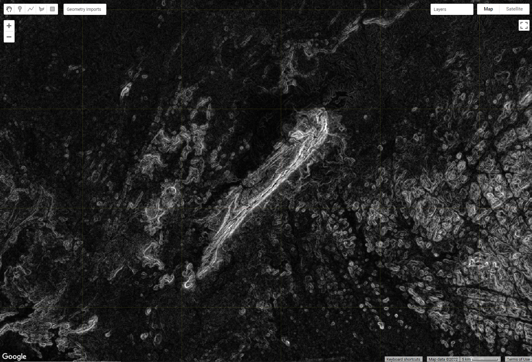
Figure 1.34: Slope image calculated with the .slope() method of the ee.Terrain package. Mount Nimba in Liberia is shown in white.
As mentioned before, there are also methods in the ee.Image container that can be invoked on an image object. We call it band math when you do mathematical operations with image bands. Still considering the previous example, suppose you are interested in further processing the slope image into an aspect image and then perform some trigonometric operations on it. Aspect, in this case, refers to the orientation of a slope, measured clockwise in degrees, from 0 to 360. Similarly to .slope(), .aspect() is also an method from ee.Terrain.
var aspect = ee.Terrain.aspect(elevationImage);Now, convert the image aspect into radians then calculate its sin:
var sinImage = aspect.divide(180).multiply(Math.PI).sin()It is worth noting that the code above chained multiple methods. This way, you can perform complex mathematical operations. In other words, the code above is simply dividing the aspect by 180 (using the .divide() method), multiplying (with .multiply()) the result of that by π (that can be retrieved using Math.PI), and finally taking the sin (with .sin()). The result should look something like the figure below:
Figure 1.35: Aspect image calculated with the .aspect() method of the ee.Terrain package. The resulting SIN image from aspect reveals Mount Nimba in greater detail.
- Band math with multi-band image
As mentioned previously, you can do mathematical operations with bands from a given image. One of the most common examples of band math with remote sensing imagery is the calculation of spectral indices. A spectral index is a mathematical equation that is applied on the various spectral bands of an image per pixel, with the objective of highlighting pixels showing the relative abundance or lack of the feature of interest. There are several categories of spectral indices that have been developed, using a variety of spectral bands to highlight different phenomena, such as water, snow, soil and vegetation. For example, Vegetation Indices (VIs) are combinations of surface reflectance at two or more wavelengths designed to highlight a particular property of vegetation.
A) NDVI
The most used index in this category is the Normalized Difference Vegetation Index (NDVI), which provides an indication of abundance of live green vegetation (or abundance of chlorophyll). The pigment in plant leaves, chlorophyll, strongly absorbs visible light (from 0.4 to 0.7 µm) for use in photosynthesis. The cell structure of the leaves, on the other hand, strongly reflects near-infrared light (from 0.7 to 1.1 µm) (See Figure 1.4). Thus, NDVI is calculated by comparing the different reflectance values of the red and near-infrared bands (normalized such that the minimum value is -1.0, and the maximum is +1.0).
Bringing this concept to the context of a Landsat 8 image, we can produce an NDVI image by computing the normalized difference between its bands 5 (near-infrared) and 4 (red) (See Figure 1.26).
For this example, we will use ImageL8 created in the previous sections to create a NDVI image. We can use the method .select() on a ee.Image object to select any given band. The .select() method will take a string as an argument for the band name you want to select. Then we can use the mathematical operators to perform a normalized difference using these bands:
var nirBand = ImageL8.select('SR_B5');
var redBand = ImageL8.select('SR_B4');
var NDVI = nirBand.subtract(redBand).divide(nirBand.add(redBand));
There is another way of doing the same calculation from the code above. As we seen previously, Earth Engine usually have methods for widely used operations and computations with remote sensing data. In this case, the normalized difference operation is available as a shortcut method .normalizedDifference() for a ee.Image() object. It take as an argument a list with the names of the bands you wish to calculate the normalized difference with. Thus, NDVI can be rewritten as:
var NDVI = ImageL8.normalizedDifference(['SR_B5', 'SR_B4'])You can then visualize this NDVI image by adding it to the Map Editor. Add it to the map and use the Inspector tab to investigate the range of values of NDVI around Cairo:
Map.addLayer(NDVI, {min: 0, max: 0.3, palette: ['a6611a', 'f5f5f5', '4dac26']}, 'NDVI Image');You should see something like this:
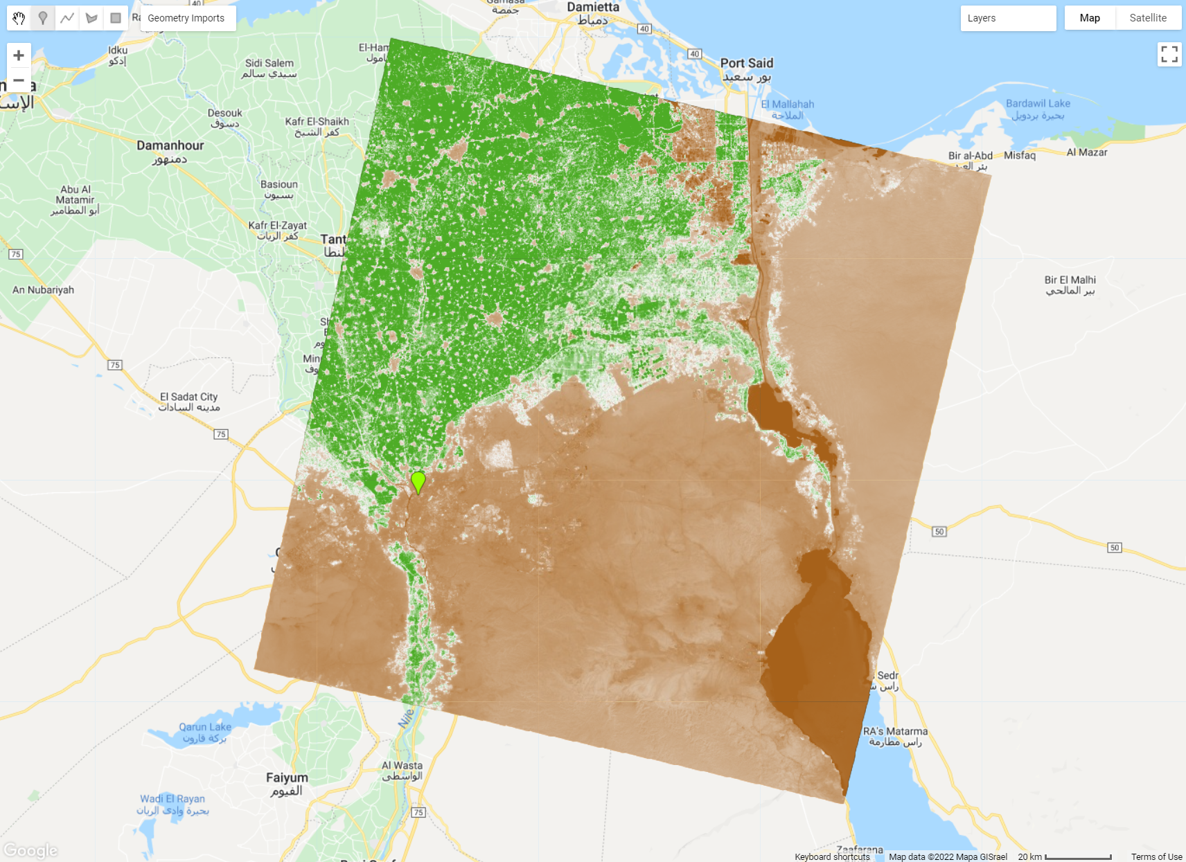
Figure 1.36: NDVI Image highlighting the agricultural area in the Nile Delta. With the visualization parameters provided above, higher values of NDVI (that is, higher content of chlorophyll in live green leaves) is shown in green.
A) EVI
EVI, or Enhanced Vegetation Index, is similar to NDVI and can be used to quantify vegetation greenness. However, EVI corrects for some atmospheric conditions and canopy background noise and is more sensitive in areas with dense vegetation where NDVI usually saturates. It incorporates an “L” value to adjust for canopy background, “C” values as coefficients for atmospheric resistance, and values from the blue band (B):
EVI = 2.5 * ((Near-infrared - Red) / (Near-infrared + C1 * Red – C2 * Blue + L)), where C1, C2 and L are usually 6, 7.5 and 1, respectively.
You can see that an expression like this can become hard to be expressed using mathematical operators such as the ones used to calculate a normalized difference. To implement more complex mathematical expressions, consider using the .expression() method for a ee.Image object. the first argument to .expression() is the textual representation (string) of the math operation, the second argument is a dictionary where the keys are variable names used in the expression and the values are the image bands to be used in the operation. Using the same ImageL8 as an example, EVI would be defined as:
var EVI = ImageL8.expression(
    '2.5 * ((NIR - RED) / (NIR + 6 * RED - 7.5 * BLUE + 1))', {
      'NIR': ImageL8.select('SR_B5'),
      'RED': ImageL8.select('SR_B4'),
      'BLUE': ImageL8.select('SR_B2')
});
The code above is able to regonize operators (+, -, *, /, %, **: Add, Subtract, Multiply, Divide, Modulus, Exponent) and the numbers; everything else is defined as keys in the dictionary.
Can you think of how you can calculate the NDVI using the code structure above?
1.2.2 Compositing and Mosaicking
Compositing is an example of a computation that can be done to a image collection. In general, compositing refers to the process of combining spatially overlapping images into a single image based on an aggregation function while mosaicking usually refers to the assembly of these images to produce a spatially contiguous one. In Earth Engine, when you composite two scenes that do not overlap completely, the resulting composite will be a composited mosaic:
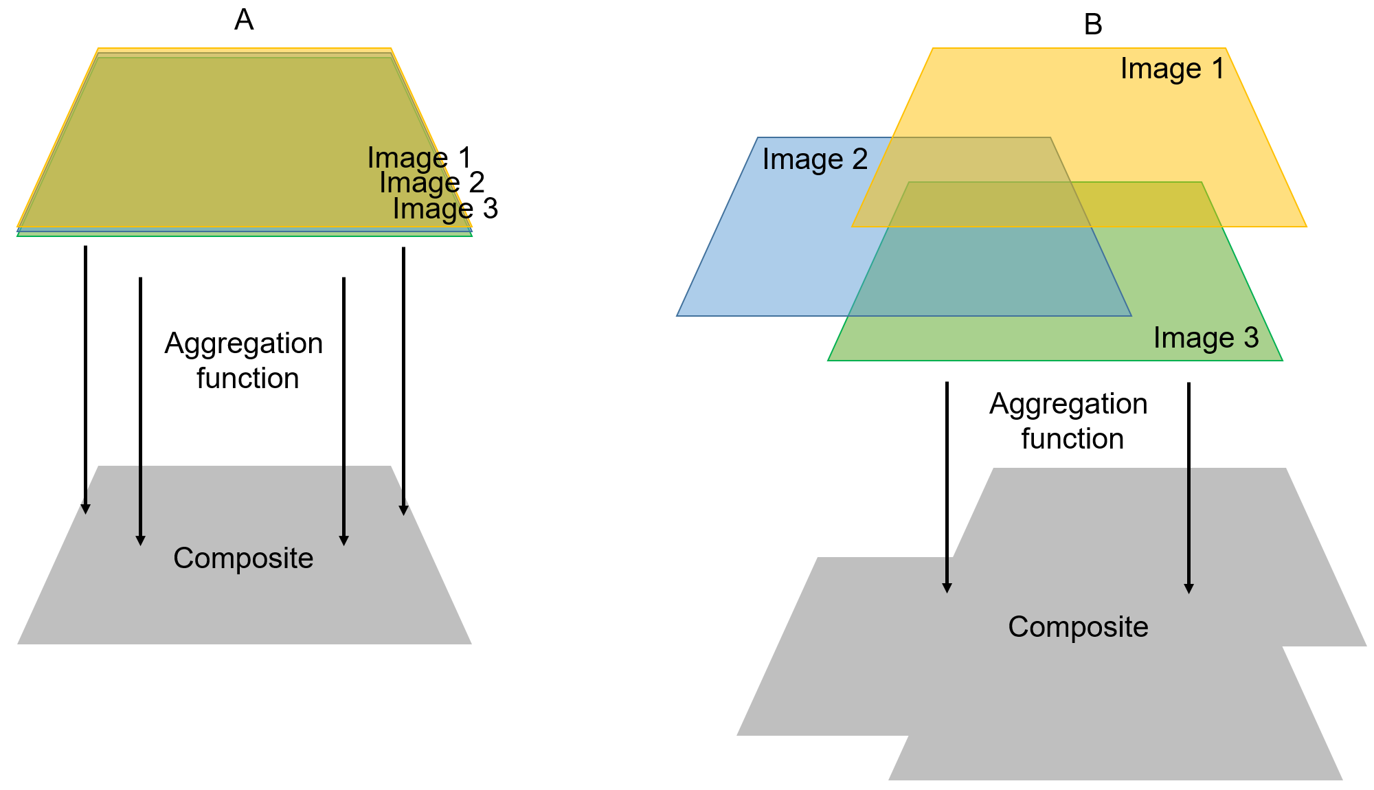
Figure 1.37: Compositing images in Earth Engine. When applying a compositing function to scenes that do not overlap completely (B), the resulting composite will be a spatially contiguous image.
Thefore, in the context of Earth Engine these terms are used interchangeably. We illustrate these concepts with the examples below.
- Example 1: Compositing the same scene (100% overlap)
In this example, we will use collectionFiltered (a Landsat 8 image collection filtered for Cairo from January to April 2022. See 1.33). There are several aggregation functions that can be used to composite an image collection, most notably .max() for a maximum value composite and .mendian() for a median value composite. All these functions will aggregate the values on a per-pixel, per-band basis. In other words, .max() will select the maximum value of a given pixel for each image band to create the final composite while .median() will calculate the median value of each band for this pixel.
var compositeMax = collectionFiltered.max();
var compositeMedian = collectionFiltered.median();
If you print these composites to the Console you will notice that they are a 19-band single image and no longer a collection with 13 images with 19 bands each!
Add these composites to the Map Editor to investigate their differences:
Map.addLayer(compositeMax, {bands: ['SR_B4', 'SR_B3', 'SR_B2'], min:8000, max:30000}, 'Composite Max');
Map.addLayer(compositeMedian, {bands: ['SR_B4', 'SR_B3', 'SR_B2'], min:8000, max:30000}, 'Composite Median');Question: What is the most evident difference between these composites?
Answer: The max value composite is mostly covered by clouds. Clouds and snow are very reflective and will always have high reflectance values for the regions of the electromagnetic spectrum covered by the Landsat spectral bands. Therefore, a maximum value composite will likely highlight these features - which is not desireable in most cases.
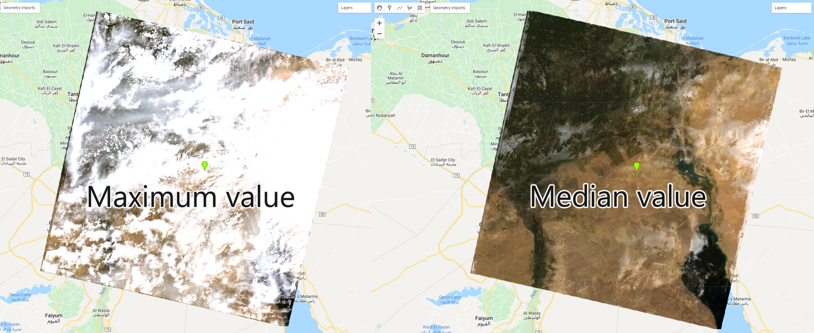
Figure 1.38: Maximum and median value composites. Clouds are evident in the maximum value composite due to their high reflectance values.
Although there are different methods for compositing, the median composite method is the state of the art in Google Earth Engine and has been applied to a multitude of studies using multitemporal remote sensing data.
- Example 2: Compositing (mosaicking) different scenes
Consider the need to composite (mosaic) four different Landsat scenes at different locations. For that we will edit the location parameter from .filterBounds() to include extra Landsat scenes from different locations. Use the information from figures 1.31 and 1.32 to create a geometry covering a larger area. Remember that .filterBounds() will filter an image collection to all the scenes that intercept the boundaries of a geometry, whether it is a line, point mark or polygon. Rename this as 'aoi2'. For this example, we will use the polygon tool to draw a large polygon over a large area in Egypt.
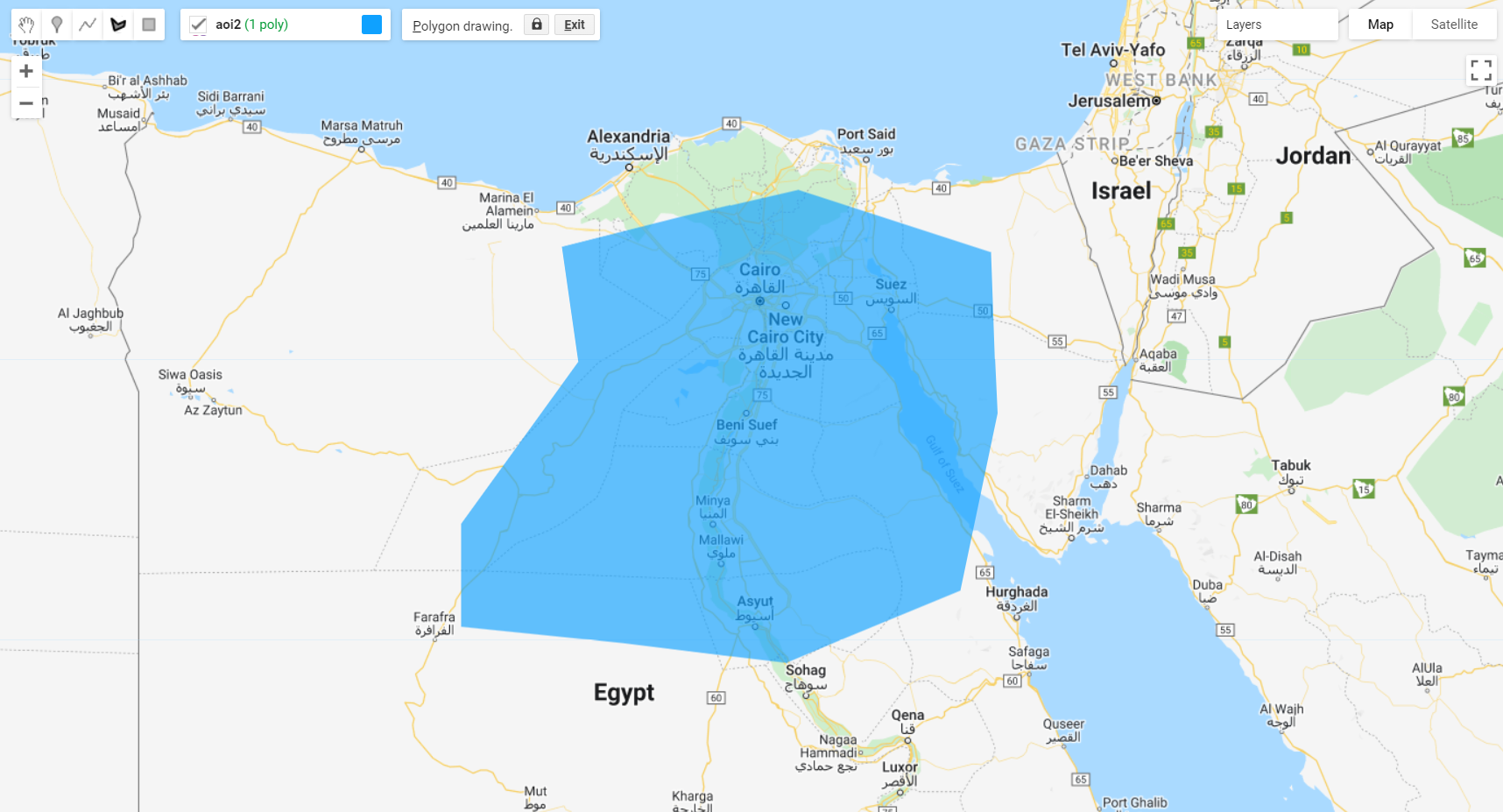
Figure 1.39: Area of interest (aoi) for filtering image collection.
We will use this geometry to filter collection to this new spatial filter aoi2:
var collectionFiltered2 = collection.filterBounds(aoi2).filterDate(startDate,endDate);
print(collectionFiltered2);
Note that if you print collectionFiltered2 to the Console you will notice that it includes more images than when we filtered for a single location using a point geometry.
Using the same compositing functions described earlier in this section, we will composite this new collection to two new composites. Also, we will use the .mosaic() method as a comparison. This method composites overlapping images according to their order in the collection (last on top):
var compositeMax2 = collectionFiltered2.max();
var compositeMedian2 = collectionFiltered2.median();
var mosaic = collectionFiltered2.mosaic();

Map.addLayer(compositeMax2, {bands: ['SR_B4', 'SR_B3', 'SR_B2'], min:8000, max:30000}, 'Composite Max 2');
Map.addLayer(compositeMedian2, {bands: ['SR_B4', 'SR_B3', 'SR_B2'], min:8000, max:30000}, 'Composite Median 2');
Map.addLayer(mosaic, {bands: ['SR_B4', 'SR_B3', 'SR_B2'], min:8000, max:30000}, 'Mosaic');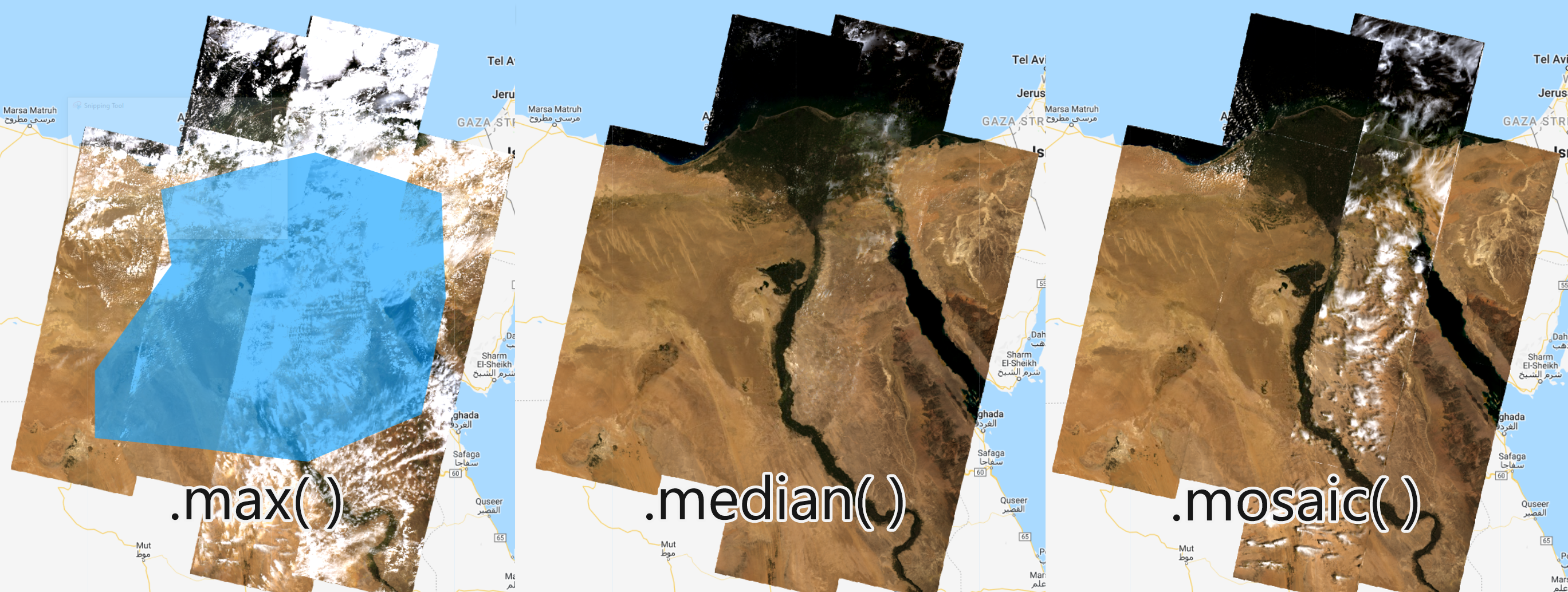
Figure 1.40: Composites of an image collection filtered by the bounds of aoi2.
Whether you are compositing using an aggregation function or mosaicking with .mosaic() the result will be similar in respect to the output type (i.e. an ee.Image object) and spatial extent. Thus, explaining why compositing and mosaicking are used interchangeably in Earth Engine.
Suppose you are only interested in the composite within the bounds of your area of interest. The method .clip() of an ee.Image() allows you to clip (or cut) any image to the shape of a geometry. We will use compositeMedian2 and aoi2 as an example:
var compositeClipped = compositeMedian2.clip(aoi2);
Map.addLayer(compositeClipped, {bands: ['SR_B4', 'SR_B3', 'SR_B2'], min:8000, max:30000}, 'Composite Median 2 clipped');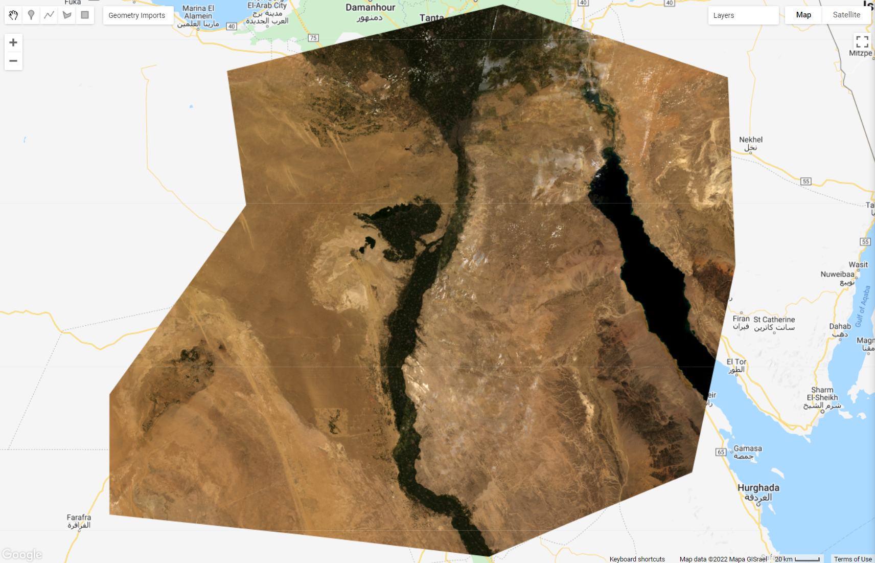
Figure 1.41: Median composite clipped by the extent of aoi2.
You can only clip an ee.Image() object, never an image collection! ``
PART 2 - Advanced Google Earth Engine
Advanced Image Manipulation: Pre-classification
In this section we will provide functions and lines of code to assist the user to prepare, process and analyze Landsat 8 data for classification purposes.
Cloud and cloud shadow masking
This sub-section demonstrates a way of masking clouds and cloud shadow pixels from Landsat 8 Surface Reflectance Collection 2 data based on file metadata. You may have noticed when exploring Landsat images in the Console tab that these images have a band called QA_PIXEL or Quality Assessment band. Briefly, this band contains values that represent bit-packed combinations of surface, atmospheric, and sensor conditions that can affect the overall usefulness of a given pixel. One of the many bits represented in this band is cloud (bit 3) and cloud shadow (bit 4):
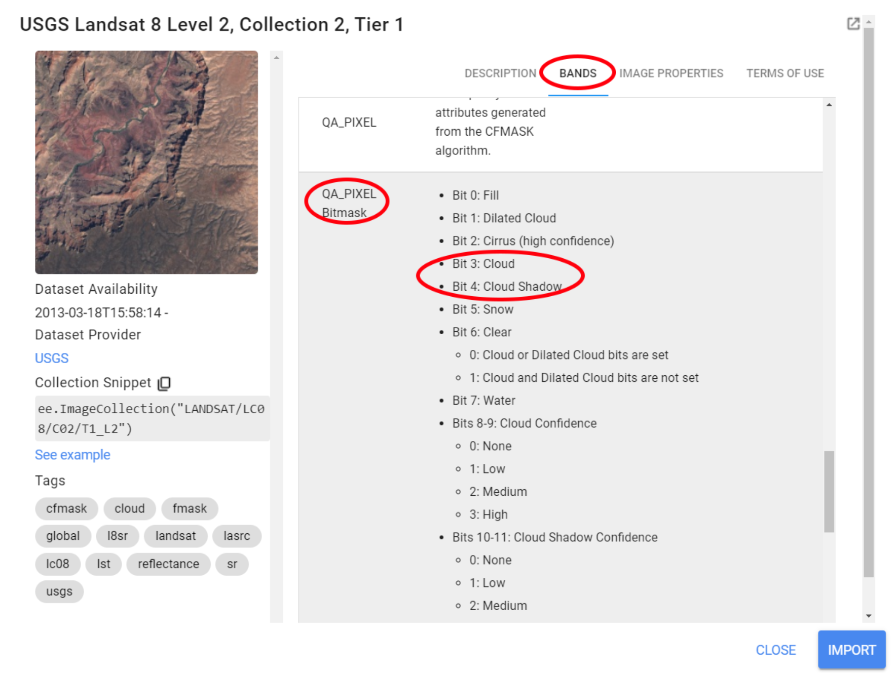
Figure 1.42: Landsat's Quality Assessment (QA) band.
In essence, these values indicate which pixels might be affected by surface conditions such as cloud contamination. Therefore, this band can be used to construct filters to mask (or remove) pixels flagged as 'affected' by that condition. Here, we will provide a function for masking clouds and cloud shadow from Landsat 8 images based on the information stored in the Quality Assessment band. This function was created based on the documentation available for Landsat 8. Values for pixel bit and pixel band were found here.
The cloud masking function is as follows:
function maskClouds(image) {
  var cloudShadowBitMask = ee.Number(2).pow(3).int();
  var cloudsBitMask = ee.Number(2).pow(4).int();
  var QA = image.select('QA_PIXEL');
  var mask = QA.bitwiseAnd(cloudShadowBitMask).eq(0)
      .and(QA.bitwiseAnd(cloudsBitMask).eq(0));
  return image.updateMask(mask).divide(100000).select("SR_B[0-9]*").copyProperties(image, ["system:time_start"]);
}
Do not worry about the new methods within this function. What you need to know is that this function was constructed in a way that we are selecting the QA_PIXEL band from the Landsat image and creating a mask where only pixels flagged to 0 (indicating clear conditions) for bits 3 and 4 will be included; The function will return image - in this case the Landsat 8 image - masked for pixels that are not flagged 0 for bits 3 and 4. The .divide() was used simply to scale the band values to [0,1] and .select() to only select the spectral bands from Landsat (SR_B1-9). These steps are not necessary for the cloud masking to work! However, we can add these extra steps to further improve our image collection.
Now, to apply a function to every image in an image collection, we use the .map() method from the ee.ImageCollection() object. You can refer to the Docs tab for more information on the methods available for ee.ImageCollection(). The only argument to map() is a function which takes one single parameter: an ee.Image(). Using .map(maskClouds) over an image collection will result in a collection where every image is masked for clouds and cloud shadows.
To illustrate this, we will apply maskClouds over collection (created in the previous chapter) along with the same temporal and spatial filters to recreate collectionFiltered. Feel free to use your previous chapter's script and simply add .map() to the collections using the code below as an example:
var collection = ee.ImageCollection('LANDSAT/LC08/C02/T1_L2');
var startDate = '2022-01-01';
var endDate = '2022-04-30';

var collectionFilteredMasked = collection.filterBounds(aoi)
                                   .filterDate(startDate,endDate)
                                   .map(maskClouds);
Now, we will create a max value composite and compare it to the previous composite created with an image collection that was not masked for clouds and cloud shadows:
var compositeMax = collectionFilteredMasked.max();
Map.addLayer(compositeMax, {bands: ['SR_B4', 'SR_B3', 'SR_B2'], min:0, max:0.25}, 'Composite Max Value');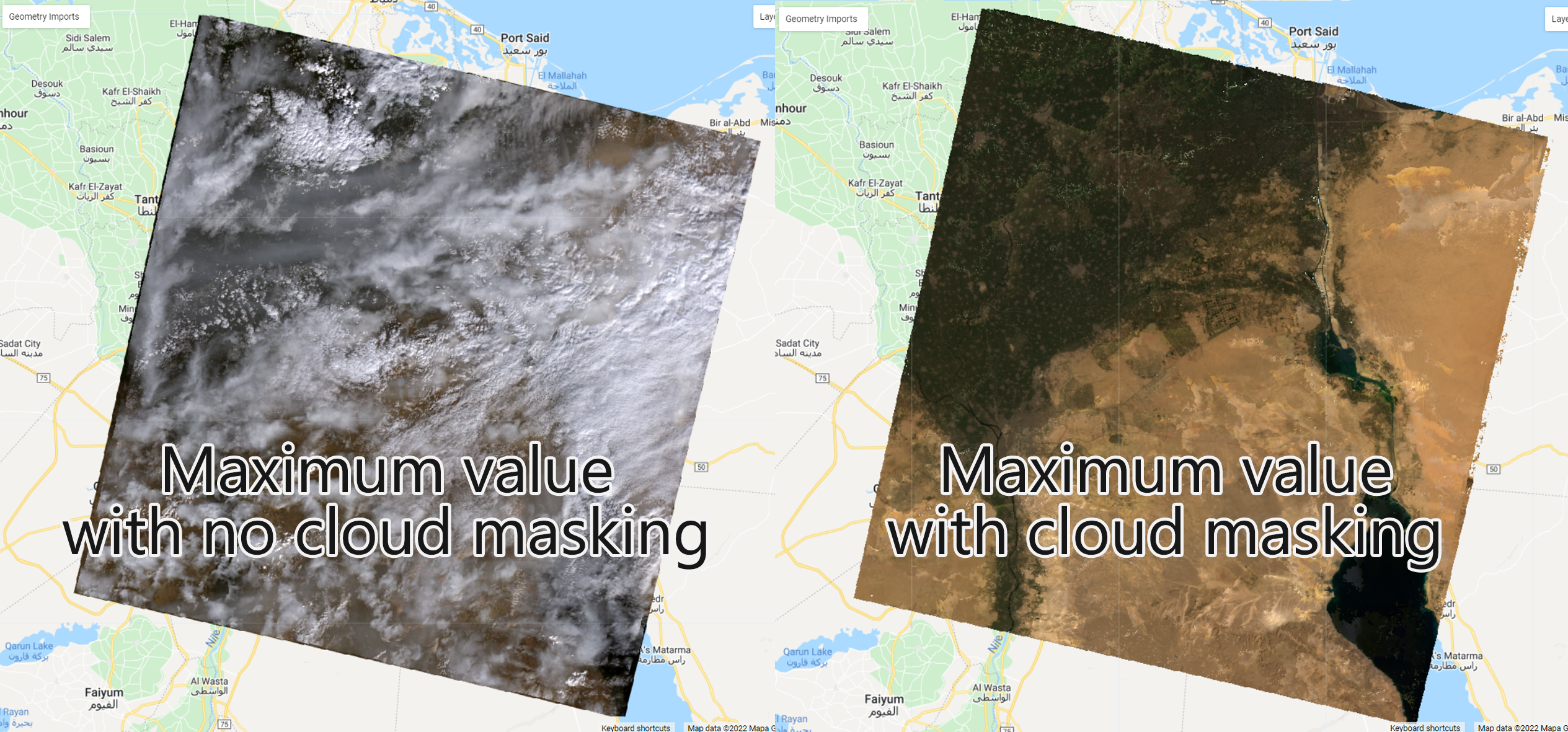
Figure 1.43: A maximum value composite created with an image collection masked by clouds compared to a composite created using an unmasked collection.
As mentioned in the previous chapter, a maximum value composite will likely highlight clouds as they are very reflective. However, by removing the cloud pixels from the images based on the Quality Assessment band information, the resulting maximum value composite greatly improves.
1.2.3 Spectral indices
In the previous sub-section, we presented a function to mask cloud and cloud shadows from Landsat image collections. A function can also be created to perform band math to every image in an image collection. Building on the concepts of vegetation indices presented on the previous chapter, we will create a function that will calculate several vegetation indices for Landsat 8 images. You will recognize the NDVI and EVI indices from the previous chapters. This function includes other commonly used spectral indices to highlight features like open water, moisture, vegetation and soil:
- NDVI - Normalized Difference Vegetation Index;
- NBR - Normalized Burn Ratio;
- NDMI - Normalized Difference Mangrove Index;
- MNDWI - Modified Normalized Difference Water Index;
- SR - Simple Ratio;
- BI - Bare soil Index;
- GCVI - Green Chlorophyll Vegetation Index;
- EVI - Enhanced Vegetation Index, and;
- MSAVI - Modified Soil-Adjusted Vegetation Index.
function addIndices(image) {
  var ndvi = image.normalizedDifference(['SR_B5','SR_B4']).rename('NDVI');
  var nbr = image.normalizedDifference(['SR_B5','SR_B7']).rename('NBR');
  var ndmi = image.normalizedDifference(['SR_B7','SR_B3']).rename('NDMI');
  var mndwi = image.normalizedDifference(['SR_B3','SR_B6']).rename('MNDWI');
  var sr = image.select('SR_B5').divide(image.select('SR_B4')).rename('SR');
  var bare = image.normalizedDifference(['SR_B6','SR_B7']).rename('BI');
  var gcvi = image.expression('(NIR/GREEN)-1',{
    'NIR':image.select('SR_B5'),
    'GREEN':image.select('SR_B3')
  }).rename('GCVI');
  var evi = image.expression(
  '2.5 * ((NIR-RED) / (NIR + 6 * RED - 7.5* SR_BLUE +1))', {
    'NIR':image.select('SR_B5'),
    'RED':image.select('SR_B4'),
    'SR_BLUE':image.select('SR_B2')
  }).rename('EVI');
  var msavi = image.expression(
  '(2 * NIR + 1 - sqrt(pow((2 * NIR + 1), 2) - 8 * (NIR - RED)) ) / 2', {
    'NIR': image.select('SR_B5'),
    'RED': image.select('SR_B4')}
).rename('MSAVI');
    return image
    .addBands(ndvi)
    .addBands(nbr)
    .addBands(ndmi)
    .addBands(mndwi)
    .addBands(sr)
    .addBands(evi)
    .addBands(msavi)
    .addBands(gcvi)
    .addBands(bare);
}
The .addBands() method is used to include an ee.Image() as a band to an existing image. Therefore, this function will calculate each index and include them as extra bands to every image in the image collection.
As in the previous sub-section, we can use .map() to map this function over collection:
var collectionFilteredwithIndex = collection.filterBounds(aoi)
                                   .filterDate(startDate,endDate)
                                   .map(maskClouds)
                                   .map (addIndices);
Then we will create median composite based on this new collection. We will add it to the Map Editor and will use the Inspector tab to explore its band values at a given location:
var compositeMedian = collectionFilteredwithIndex.median();
Map.addLayer(compositeMedian, {bands: ['SR_B4', 'SR_B3', 'SR_B2'], min:0, max:0.25}, 'Composite Median');
You can toggle the data view from chart to values with the chart/value view button:
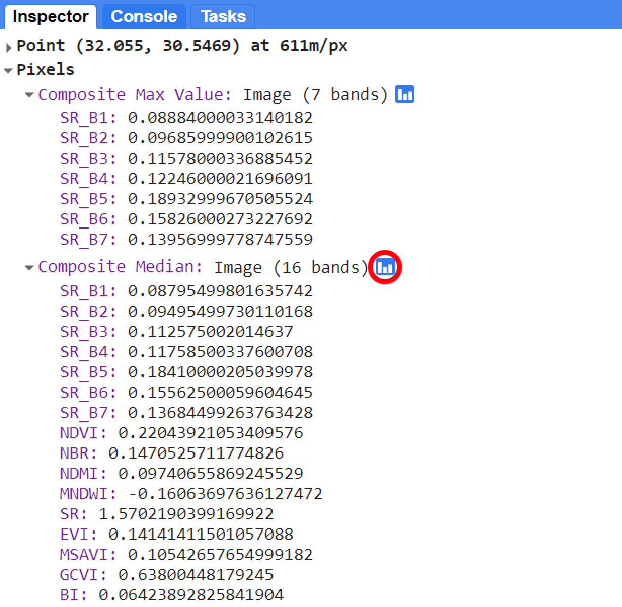
Figure 1.44: A median composite created from the collectionFilteredwithIndex image collection. The function addIndices was used to calculate each index and add them as separate bands to every image in the collection. In this example, the spectral bands and spectral index values for a pixel at an arbitrary location within compositeMedian. You can toggle between the chart view and value view using the chart button (red circle).
1.3 Supervised Classification using Random Forest
As seen in Part 1, Interpretation and Analysis is one of the building blocks of any remote sensing system (see 1.1). Image classification is one of the many methods of image processing and it is the sole focus of this training material. So far, you have learned the basics of Java Script and Google Earth Engine and some pre-processing steps to perform an image classification using the Random Forest (RF) Classifier. Briefly, classifier is an ensemble of classification trees, where each tree contributes with a single vote for the assignment of the most frequent class to the input data. Different from Decision Trees, which use the best predictive variables at the split, RF uses a random subset of the predictive variables. To illustrate this concept, we will use a rather simplistic example:
Suppose you were given this list of attributes from three edible fruits:

Figure 1.45: Simplistic list of predictive variables from three types of fruits.
A random forest classifier can be created (or trained) using the sample above as a training sample set:

Figure 1.46: A Machine Learning Random Forest Classifier with 3 trees trained with the sample set above. Note that algorithm was able to 'learn' about each fruit separate them based on their attributes.
You can test this classifier and its accuracy using a testing sample set. A testing set is usually a subset of the training set that will be used only for testing the performance of the trained classifier. These testing samples will be run through each tree of the ensemble and the accuracy of the classifier will be based on whether or not it was able to classify that sample correctly:
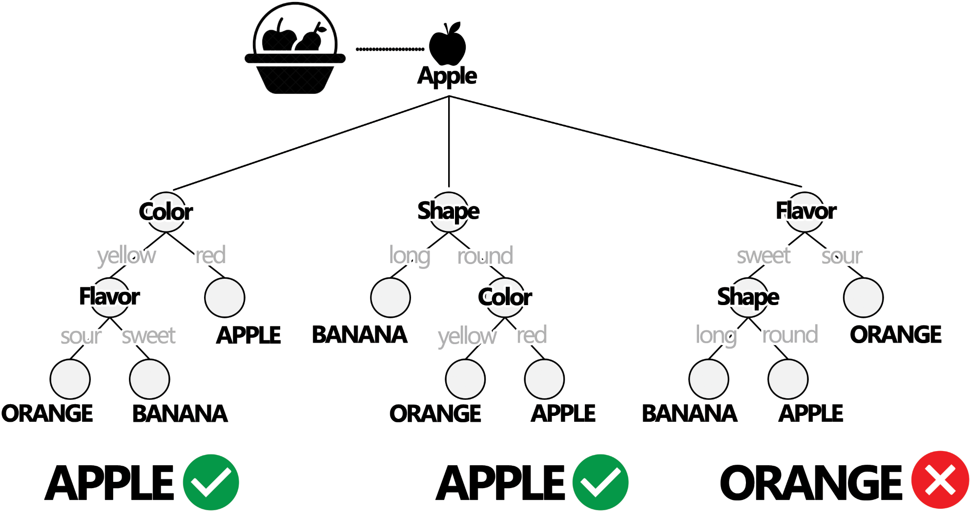
Figure 1.47: Testing a trained Random Forest Classifier. A testing sample is used to assess whether or not the classifier is able to correctly classify them. In this example, this sample was correctly classified by 2 out of the 3 trees in the ensenble.
You can then classify unlabeled samples using the trained classfier. The final classification of a sample is based upon the majority of the votes of the trees in the ensemble:
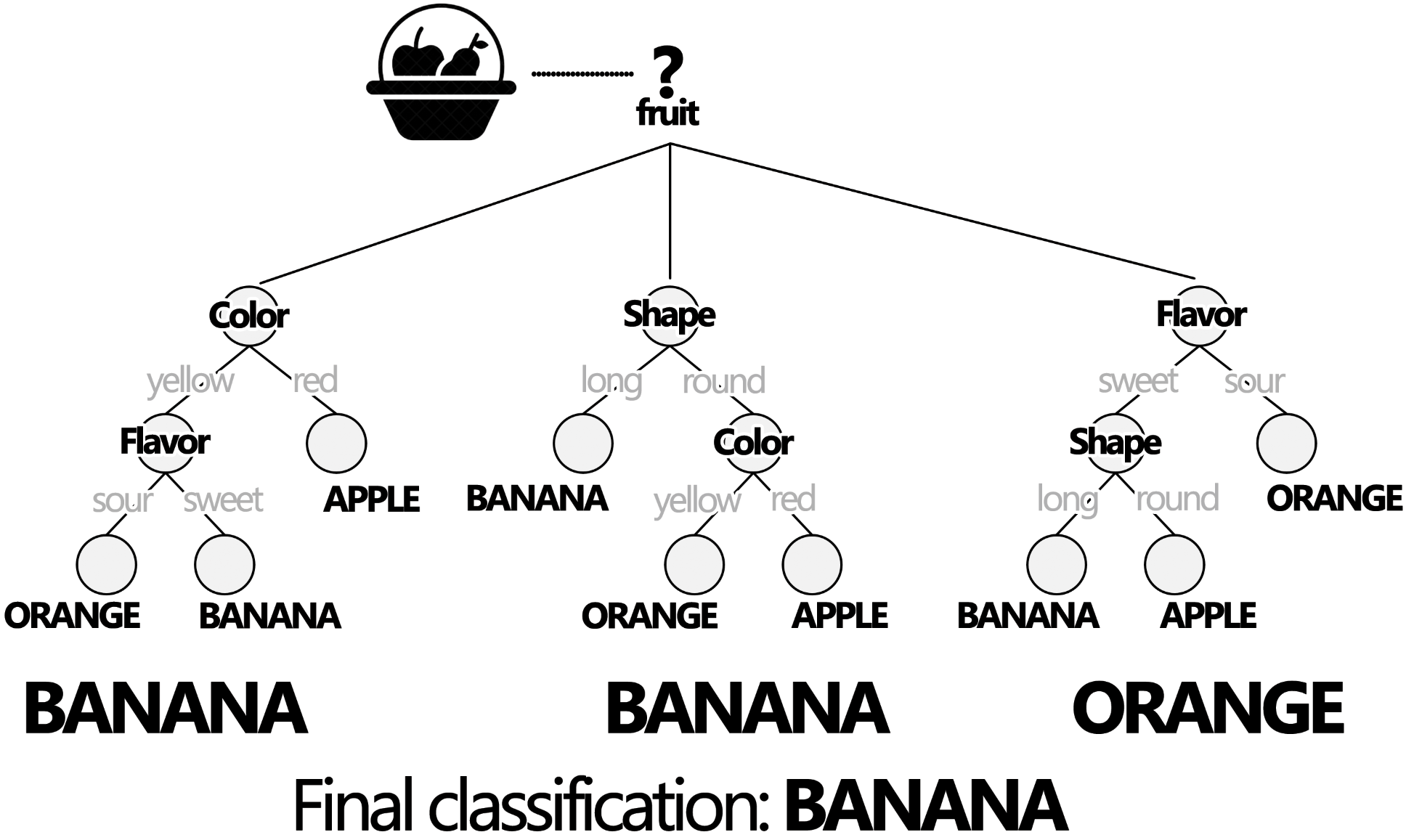
Figure 1.48: The trained RF classifier is used to classify an unlabeled fruit sample. In this case, the majority of the votes (2 out of 3) was BANANA. Therefore, the final classification of this sample is BANANA.
Even though this is a rather simplistic example, it can be easily translated into a land cover classification context: Instead of fruits, each unit being classified is a Landsat image pixel. Each pixel from each land cover class will contain different spectral attributes. These spectral attributes will be used at each branch of the trees in the ensemble. We can then used a trained Random Forest classifier to label hundreds of thousands Landsat pixels into different land cover classes. The RF is one of the most used and robust classifiers and it is fully implemented in GEE. In the following examples we will present the steps for land cover classification using the RF classifier and present some basic analysis that can be done using the classification output.
1.3.1 Example 1: Land cover classification of Greater Cairo and Giza area, Egypt - Year 2022
The general steps for an image classification process with Landsat image is:
To use a cloud-masking function to mask clouds on Landsat 8 Imagery;
To calculate spectral indices that will be used as predictors for the Random Forest;
To produce a cloud-free composite mosaic using the median reducer, and;
To select training samples;
To classify the cloud-free composite mosaic of Landsat 8 scenes using Random Forest.
In this example we will classify the median composite (compositeMedian) created in the previous section. You can find the code for creating it here.
You have the option to classify the entire scene or clip it to an area of interest. You can create a geometry AreaOfInterest and clip your composite using .clip(AreaOfInterest). You can also customize the composite visualization parameters by clicking on the settings icon (gear ⚙) next to the layer name (in this example: 'Composite Median')
So far, we have covered the steps a, b and c.
- Training sample selection
For this example, let’s classify the 'composite' into four classes: water, agricultural land, sand and bare areas and urbanization. The first step is to create the training samples set to use into the Random Forest Model.
Step 1 - In the Geometry Imports, click +new layer and make four sets of geometries, each set will represent samples from the classes 'water', 'cropland', 'sand', and 'urban'.
Figure 1.49: Geometry sets to hold samples for each of the four classes.
Step 2 - For each geometry in the list, click on the settings icon⚙: name them accordingly using the 'Name' box, choose a color for it using the color picker and import each geometry as FeatureCollection. Add a property called landcover by clicking on the + Property and set a consecutive integer starting from 0 or 1 for each of the classes. You should achieve something similar to this:
Figure 1.50: Geometries used to create the training sample sets.
Your Geometry Imports should look like this:
Figure 1.51: Geometry Imports after creating geometry sets to hold training samples
Start selecting samples by clicking on the ‘Water’ geometry in the Geometry Imports. Choose the point drawing tool and place some points along the River Nile:
Take advantage of the high resolution imagery to help you select samples for each class. You can toggle in between map and Google Earth imagery by using the buttons Map and Satellite in the upper right corner of the Map Editor. You can also toggle the Landsat composite ON and OFF by using the layer manager.
Instead of single points (i.e pixels), we can also use polygons containing a variable number of relatively homogenous pixels of a given land cover class. Switch to the polygon drawing tool and draw a few polygons over the River Nile:
Figure 1.52: Sample points and polygons for the Water class
Once you finish selecting samples, click the Exit button on the polygon editor dialogue box . Repeat the process for each of the other class. Make sure you select samples that are representative of each land cover class by selecting points and polygons of homogenous pixels.
Figure 1.53: Example of sample points and polygons for ‘Water’ (blue), ‘Cropland’ (yellow), ‘Urban’ (red) and ‘Sand’ (pink). Each pixel within the polygons will be used as training inputs for the RF classifier.
After selecting the samples, we will merge all the geometries together into an object var classes using the .merge method of the ee.FeatureCollection() object:
var classes = Water.merge(Cropland)
                   .merge(Sand)
.merge(Urban);- Sample sets
In this section, we will create the training (and testing) sample sets to be used in the classification with Random Forest. First, we will select the predictors to assign to each sample point in the sample sets. For this example, we will create a list 'bands' with the names of three spectral bands ('SR_B4','SR_B5','SR_B6') and the spectral indices ('NDVI','NBR','MNDWI','SR','GCVI' and 'MSAVI').
var bands = ['SR_B4','SR_B5','SR_B6','NDVI','NBR','MNDWI','SR','GCVI','MSAVI'];Next, we will sample the Landsat pixels by overlaying the geometries with the composite using .sampleRegions(). The main arguments of this method is the image to sample (in this case, compositeMedian), the regions to sample over (in this case, classes) and the list of properties to copy from each geometry (in this case landcover):
var samples = compositeMedian.select(bands).sampleRegions({
  collection: classes,
  properties: ['landcover'],
  scale: 30
}).randomColumn('random');
In the samples object we have just created, each sample will include a column with the values from the list bands inherited from the compositeMedian and a column with their respective class label. Optionally, you can perform an accuracy assessment of the classifier by taking advantage of the identifiers assigned to the samples by the .randomColumn('random') within samples. This method adds a column to the feature collection populated with random numbers in the range of 0 to 1. For this example, we will randomly partition the sample set into training (80% of the samples) and testing (20% of the samples) samples by filtering the samples by its random number column using the lower (.lt) and greater than or equal (.gte) filters:
var split = 0.8;
var training = samples.filter(ee.Filter.lt('random', split));
var testing = samples.filter(ee.Filter.gte('random', split));
For your information, you can inspect the size of a ee.FeatureCollection using the .aggregate_count() method. This method only takes a property of the feature collection being counted as its argument. In this case, we have a property called 'landcover' in our feature collection. .aggregate_count() It is a useful tool to extract the number of features on your sample set:
print('Samples n =', samples.aggregate_count('landcover'));
print('Training n =', training.aggregate_count('landcover'));
print('Testing n =', testing.aggregate_count('landcover'));
If a feature collection do not have a property defined, you can still count its feature by using '.all' as an argument for .aggregate_count().
Using the split value above, roughtly 80% of the features in samples will be training and 20% will be in testing:
Figure 1.54: Sample sets size for this example. Note that the number will vary based on the number of geometries (polygons and points) and the sample split value.
- Classification
Next, we will train a Random Forest classifier using the training sample set training. The Random Forest classifier ee.Classifier.smileRandomForest has several user-defined parameters. However, two of them are the most usually defined: the number of trees in the ensemble (a.k.a ‘forest’) and the number of predictors to randomly tested at each tree. Predictors, in this case, are the spectral bands and spectral indices associated to each training sample. If unspecified, it uses the square root of the number of predictors.
Higher number of trees and number of predictors tested at each node do not mean better performance and overall accuracy.
For this example, we will use 200 trees and 8 randomly selected predictors to use in each tree and train Random Forest model called 'classifier' using the .train() method on the .ee.Classifier.smileRandomForest():
var classifier = ee.Classifier.smileRandomForest(100,5).train({
  features: training,
  classProperty: 'landcover',
  inputProperties: bands
});
In the features argument of the code above, make sure to select the predictors you want to use from the sample set (in this example, training) to train the model. In this case we are providing all of them. However, if you want to select a particular group of variables, you can use .select(['variableName1','variableName2',..]). Also, you must include the class property (classProperty) in which the class label is stored (in this example 'landcover').
You can test the accuracy of classifier by classifying the testing samples using .classify() method. Then, you can compute a 2D error matrix for the classified testing samples using .errorMatrix(). This method will output an ee.ConfusionMatrix() object by comparing the two columns of the classified testing samples: one containing the actual labels (in our case, the property called 'landcover'), and one containing predicted values by the classifier (which defaults to 'classification'). Finally, you can use .accuracy() method of the ee.ConfusionMatrix() object to compute the overall accuracy of the classifier:
var validation = testing.classify(classifier);
var testAccuracy = validation.errorMatrix('landcover', 'classification');

print('Validation error matrix RF: ', testAccuracy);
print('Validation overall accuracy RF in %: ', testAccuracy.accuracy().multiply(100));
As explained earlier, the trained classifier can be used to classify the compositeMedian. Google Earth Engine will run each pixel through each of the 200 trees in the classifier and assing it the label which had the majority of votes among all the tree:
var classification = compositeMedian.select(bands).classify(classifier);For visualization of the resulting classification output, we will create a color palette object paletteMAP with a list of colors for each class of the map. The order of the colors in the palette will follow the order of the classes:
var paletteMAP = [
  '#0040ff',  // Water (Class value 0)
  '#00ab0c',  // Croplands / Cultivated Areas (Class value 1)
  '#fbf2ad',  // Sand and bare areas (Class value 2)
  '#878587'   // Built-up and Urban Areas (Class value 3)
];
Finally, we will add classification to the map using Map.addLayer(): use min: 0 (first class), max: 3 (last class), add the color palette paletteMAP and a name for the layer:
Map.addLayer (classification, {min: 0, max: 3, palette:paletteMAP}, 'Classification');After several seconds, you should see something similar to the figure below:
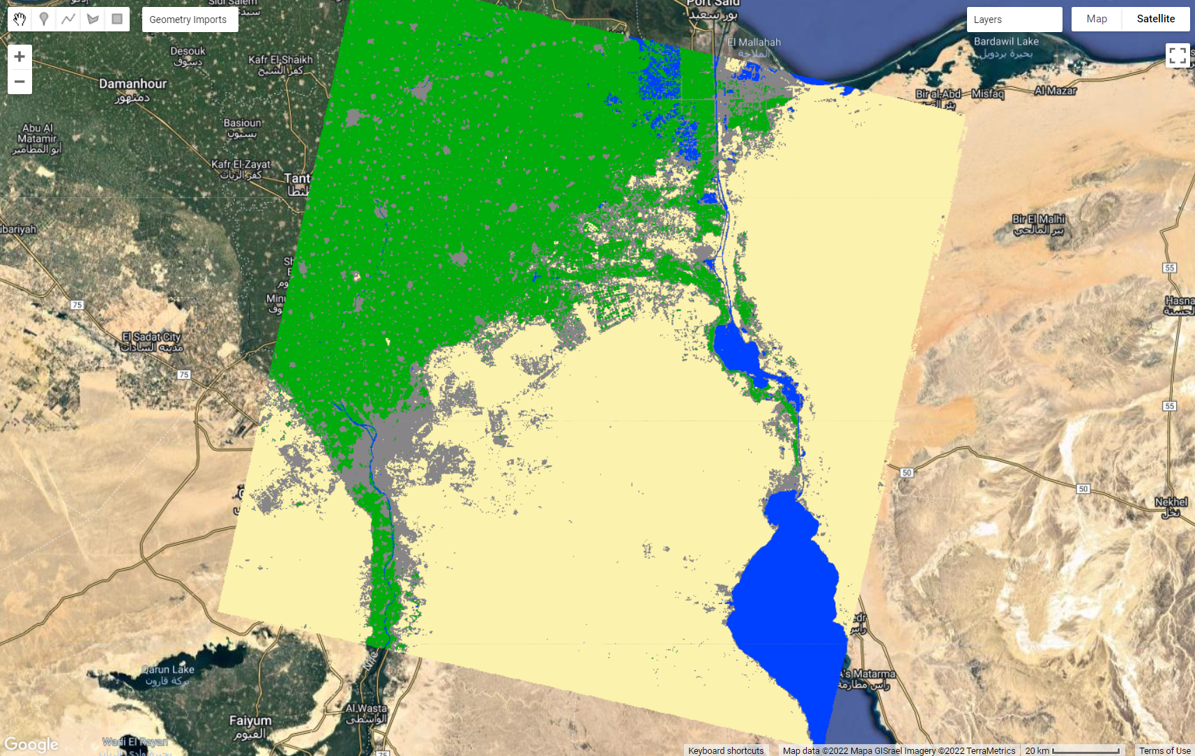
Figure 1.55: Random Forest classification output for 2022.
As an optional step, you can export your classification output as a Google Earth Engine asset. You can save geospatial datasets and analysis outputs into your Google Earth Engine account through the Assets tab and the left side of the code Editor.
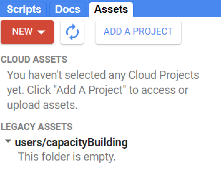
Figure 1.56: Assets manager. Your Google Earth Engine account will be able to host around 200GB worth of assets. Externally imported assets as well as datasets exported from Earth Engine scripts will be found here.
You can also upload external datasets into your Google Earth Engine Assets with the NEW button. (See Earth Engine's Importing Raster Data for instructions on uploading an image to your assets or Importing Table/Shapefile Data for more details).
We will export classification with the Export.image.toAsset() method. This method takes a dictionary with several parameters such as:
image: the image object you want to export;description: a description to be showing on the Task tab. No spaces allowed;assetId: A name for your asset. No spaces allowed;scale: A scale to export;region: the region or area of yourimageyou want to export. It takes a geometry/ feature collection;maxPixels: This is somewhat important argument. In order to avoid memory errors, the Earth Engine detault is 1x10e8 pixels. If you do not define your max pixels and your exports exceeds the default, you will get an error.
We will create a geometry 'region' to encompass the entire classified scene in order to export the entire area. The code below will export the classification:
Export.image.toAsset({
  image: classification,
  description: 'ClassificationOutput',
  assetId: 'Cairo2022',
  scale: 30,
  region: region,
  maxPixels:1e12
});
Running the code above, will create the exporting task named ClassificationOutput in the Tasks tab.
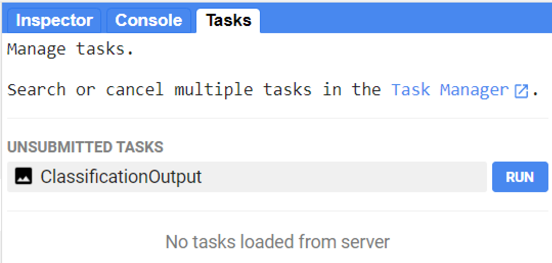
Figure 1.57: Tasks manager.
Clicking the Run button will start exporting your classification. You can check some of the parameters of the Export.image.toAsset() one more time before exporting the asset. You are allowed to change some of these parameters at this point. For our example, everything will follow the parameters we defined previously.
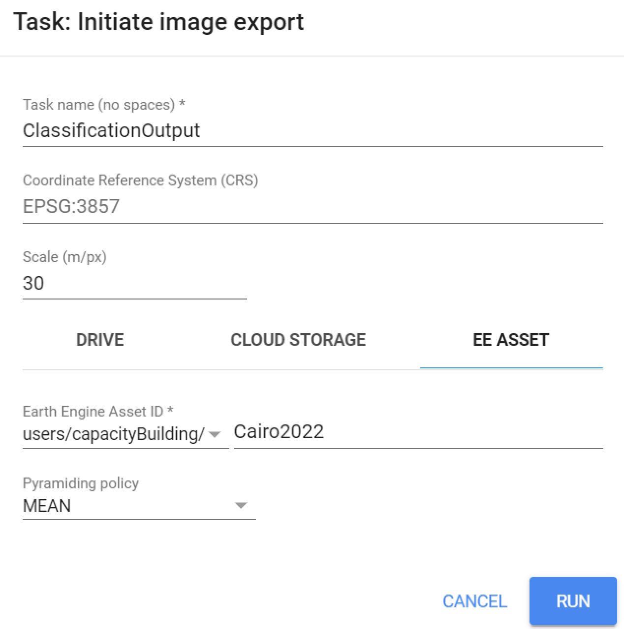
Figure 1.58: Tasks manager: Image Export.
The time elapsed of your exporting task will be shown in the Tasks tab.

Figure 1.59: Once a task has started the time elapsed will be shown in the Tasks tab.
I may take several minutes to export your classification image to your assets. Once your task is completed, it will be shown at the Task tab as:

Figure 1.60: Exported asset.
Finally, your export will be available as an Earth Engine asset:
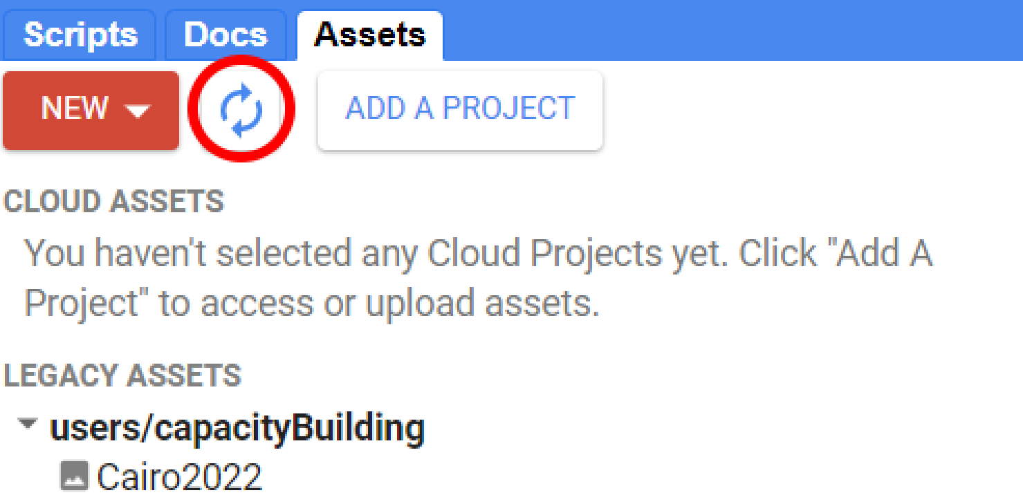
Figure 1.61: Assets will be available through the Assets tab. If they are not showing, try refreshing the folder with the refresh button.
1.3.2 Example 2: 2015 - 2022 Map-to-Map change of greater Cairo and Giza area, Egypt
In this example, we will use the codes from Example 1 to create a land cover classification for the year 2015 period. Following are the changes to be made on the codes from Example 1:
- The
yearobject will have a value of'2015'; - Repeat the training sample selection to make sure the samples reflect the correct land cover class for the L8 composite in the year 2015.
You can access the edited script for two steps above here.
After following the 2 steps above, you should achieve a similar output as before:
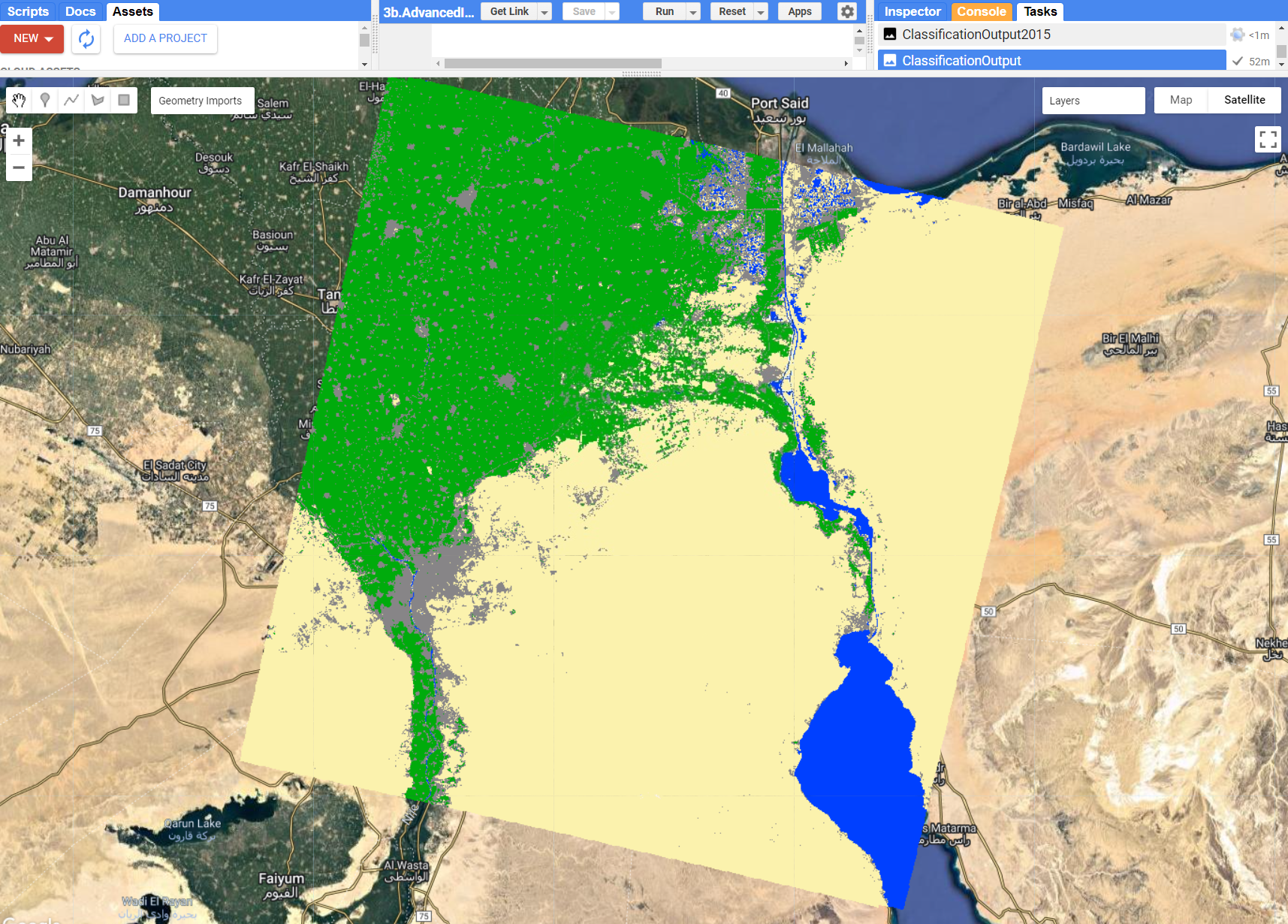
Figure 1.62: Random Forest classification output for 2015.
Export this new classification to you assets. Next, open a new code editor page and add the classification exports to this script by clicking the Import into script button (blue arrow) for both classification assets in the Assets tab:

Figure 1.63: Assets tab with classification maps. Clicking in the Import into script button will add the assets to the script.
Finally, rename each import by clicking on their names at the Imports header:

Figure 1.64: Imports header. You can rename imported assets by clicking on its name.
Alternatively, you can import assets to your scripts by using ee.Image() and their respective asset directory. For this example, you can use:
var Cairo2015 = ee.Image("users/capacityBuilding/Cairo2015");
var Cairo2022 = ee.Image("users/capacityBuilding/Cairo2022");
Add Cairo2015 and Cairo2022 to the map using the code below:
var paletteMAP = [
  '#0040ff',  // Water - pixel value = 0
  '#00ab0c',  // Croplands / Cultivated Areas - pixel value = 1
  '#fbf2ad',  // Sand and bare areas - pixel value = 2
  '#878587',  // Built-up and Urban Areas - pixel value = 3
];

Map.addLayer(Cairo2015, {min: 0, max: 3, palette:paletteMAP}, 'Cairo2015');
Map.addLayer(Cairo2022, {min: 0, max: 3, palette:paletteMAP}, 'Cairo2022');
You can examine both layers on the map and try to identify areas where classes have changed in the 7 years period. However, we can use a transition error matrix to quickly quantify these changes. This matrix can be used to assess how much each class has changed and to what they have changed based on sampling design of your choosing. To do that, we will start by stacking both maps Cairo2015 and Cairo20222 into a single object stackedClassifications and rename Cairo2015 and Cairo2022 as 'before' and 'later', respectively:
var stackedClassifications = Cairo2018.rename('later').addBands(Cairo2000.rename('before'));Next, we will create a testing sample set with 1000 points for each class using a stratified random sampling design. In this sampling design each class has the same weight. Therefore, the same number of points will be placed in each class, regardless of its relative extent. This is important to consider as some classes may have very small area extent to be captured by a random sampling design. In this example, water bodies is relatively small compared to the other three land cover classes. Thus, a stratified sampling design will ensure that this class will have the same number of points. We can used .stratifiedSample() method. This method takes a dictionary with several parameters such as:
numPoints: Number of points you want to select by each class;classBand: The classification you want the sample points to inherit the class labels from;scale: Always remember to set the scale to match Landsat nomimal spatial resolution (30 m)
Always remember to check the Docs tab for more information on the parameters each method takes!
Using the information above, a stratified sample set can be created as following:
var samples = stackedClassifications.stratifiedSample({
numPoints: 1000,
classBand: "before",
scale: 30,
geometries: true
});
Once the points are placed, they will inherit the class label (pixel value) from Cairo2015 ('before'):
We can add the samples to the map using Map.addLayer(). To colorize geometries, you use the color paramenter instead of palette:
Map.addLayer(samples, {color:'black'}, 'Stratified samples');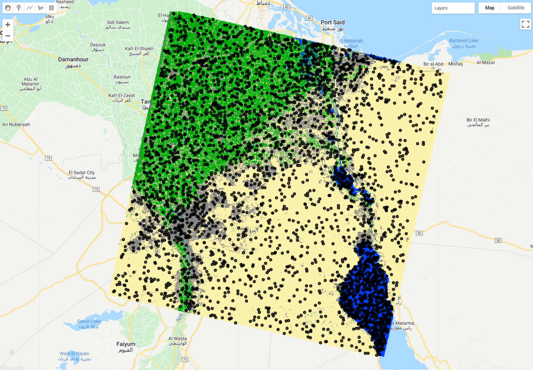
Figure 1.65: Stratified samples. 1000 samples were randomly selected within each strata (class).
Next, we will create a transition matrix using the samples above. This matrix will show how many of these 1000 remained the same land cover class 7 years later (Cairo2022) and how many of them changed to a given class. You can use .accuracy() to calculate the % of these samples remained unchanged between the two periods:
var transitionMatrix = samples.errorMatrix({
  actual: 'before',
  predicted: 'later'
});

print('Transition Matrix', transitionMatrix);
print('% of Unchanged Samples: ', transitionMatrix.accuracy().multiply(100));
The matrix will be printed to the Console tab. The code above should produce something similar to figure below:
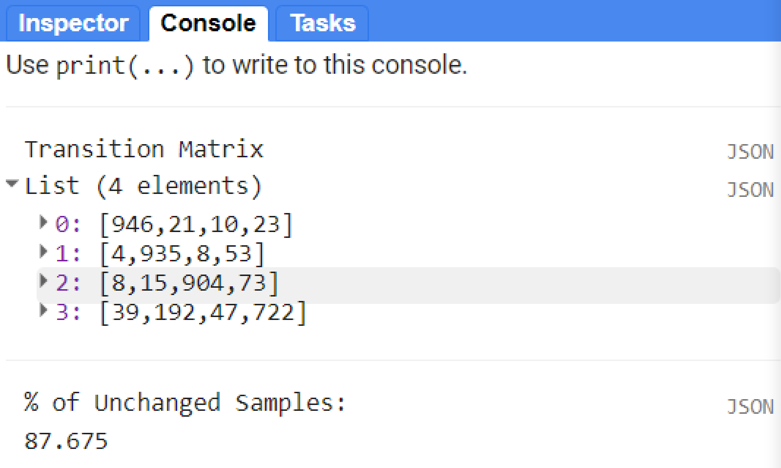
Figure 1.66: Transition matrix based on the 4000 (1000 for each class) samples.
In the transition matrix above you can draw information about how many samples transitioned to each class from 2015 to 2022. For example, from the 1000 samples of agriculture class (pixel value 1), 4 was classified (or ‘transitioned’) to water, 8 to sand and 53 to urban areas in 2022. 935 of them remained unchanged. Overall, 87% of these samples from all classes remained unchanged.
- Cropland area expansion and conversion in the Nile Delta from 2015-2022
Another quick analysis that can be done with land cover class maps in two points in time is highlighting areas in which a particular class has changed. In this example, we will assess the cultivated/cropland change between the 2015 and 2022. First, we will isolate the agricultural land class (pixel value 1) from both years into separate objects class2015 and class2022 using the .select() and .eq() methods. Secondly, we will calculate the change by simply subtracting both objects:
var class2015 = Cairo2015.select(['classification']).eq(1);
var class2022 = Cairo2022.select(['classification']).eq(1);
var change = class2022.subtract(class2015);
By default, the new objects class2015 and class2022 will have values of 1 where the 'classification' has the label equals (.eq) to 1 (agriculture) in the land cover map. This will be the case regardless of the label value. By using the .select() and .eq(), the new image object will default to value of 1 where that condition was met. Thus, the object change will have values of -1, 0 and 1, that represents loss/conversion, no change and gains, respectively:
-1= No crops in 2022 - crops in 2015 (0 - 1 = -1);0= crops in 2022 - crops in 2015 (1 - 1 = 0);1= crops in 2022 - no crops in 2015 (1 - 0 = 1)
We will add change to the map.
var paletteCHANGE = [
  'red',    // Loss/conversion
  'white',  // No Change
  'green',  // Gain/Expansion
];

Map.addLayer(change, {palette: paletteCHANGE}, 'Change 2015-2022');
The resulting change map will look similar to figure below. Green pixels represent 'gains' while red pixels represent 'conversions':

Figure 1.67: Subset of the 2015-2022 Change Map. Conversion/loss of classifiedagricultural areas.
This code can easily be used to investigate the other classes as well. Simply change the class value within .select(['classification']).eq(classValueHere).
In the example below, we changed the value from 1 to 3 to highlight the expansion of urban/built up areas.

Figure 1.68: Subset of the 2015-2022 Change Map. Expansion of the future capital of Egypt, New Cairo City.
You can calculate the area of expansion/conversion by isolating the pixels of gain/loss from the change object into gain and loss. Then, calculate the area of each pixel using ee.Image.pixelArea() and multiplying by the count of pixels in gain and loss using multiply. The default unit is square meters (m²). You can use .divide() to transform into square kilometers (.divide(1000000)) or hectares (.divide(10000)):
var gainArea = gain.multiply(ee.Image.pixelArea().divide(1000000));
var lossArea = loss.multiply(ee.Image.pixelArea().divide(1000000));
These objects will hold the area calculation for a single pixel. Then, we can use .reduceRegion() method, from the ee.Image() container. This will apply a reducer to all the pixels in a specific region. This method will take the reducer parameter, which will contain the type of mathematical operation you wish to compute for all these pixels. In this case, we will use ee.Reducer.sum(), to sum up all the single area values for all the pixels within gainArea and lossArea:
Make sure to create a geometry around an area of interest in order to calculate the area (extent) for the pixels of a given class within that geometry! In this example, we used a geometry around New Cairo City called 'AOI'.
var statsgain = gainArea.reduceRegion({
  reducer: ee.Reducer.sum(), // Sum of all the area values.
  scale: 30,                 // Landsat scale.
  geometry: AOI,
  maxPixels: 1e14
});

var statsloss = lossArea.reduceRegion({
  reducer: ee.Reducer.sum(),
  scale: 30,
  geometry: AOI,
  maxPixels: 1e14
});
Finally, you can print these values using the code below:
print(statsgain.get('classification'), 'km² of new built up areas in New Cairo City'); 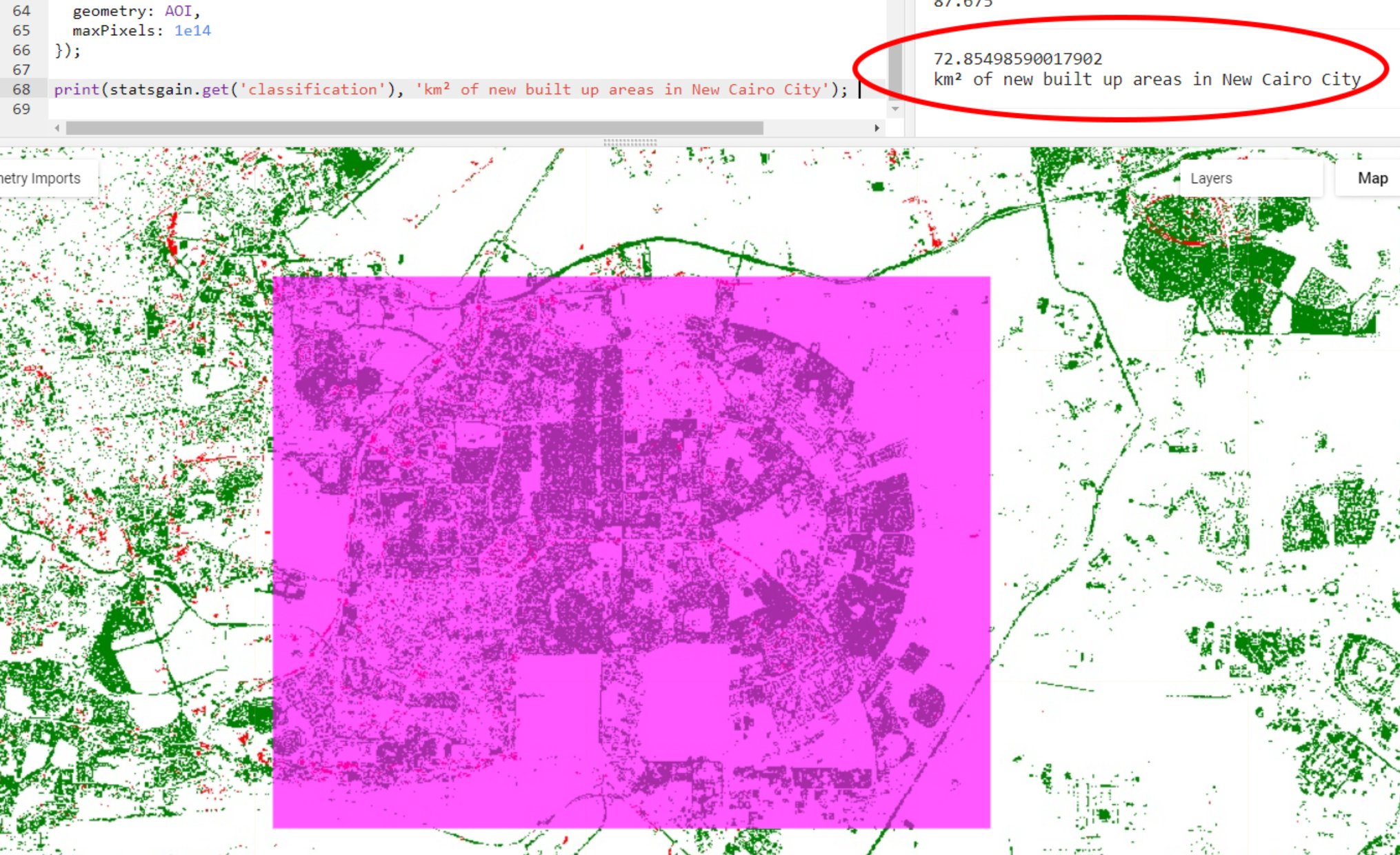
Figure 1.69: Subset of the 2015-2022 Change Map. Expansion of the future capital of Egypt, New Cairo City. The .reduceRegion() method was used to calculate the extent of gains for the urban/built up class. Finally print() was used to print the result to the Console tab.
1.4 Post-classification processing
So far you have learned the basics of creating a classification output using a machine learning algorithm such as Random Forest. The objective of this section is to provide useful post-classification steps for corrections and general improvement of a random forest classification output.
1.4.1 Re-classification
Classification outputs often times will need some degree of correction or adjustment. Some of these corrections and adjustments include, for example, the Correction for missclassification erros in specific areas and changing class labels (pixel values) or class order. In this section we will explore the function remap(). This function maps from input values to output values, represented by two parallel lists: one includes the original number of classes and their value; the other represents which class (or classes) is being remapped and what it is being remapped to. To ilustrate this concept, consider the following example:
- The previously produced land cover maps include four classes: Water (pixel value = 0), Cropland / Cultivated Areas (pixel value = 1), Sand and bare areas (pixel value = 2) and Built-up and Urban Areas (pixel value = 3) (List 1). If any of these class values needs to be changed, the new value for that class is placed in the List 2, in the position of the class that needs changing (Figure 1).
Figure 1.70: The remap function for the land cover classification of the Greater Cairo.
To test this function, start by opening a new code editor page and importing one of the classification assets you used in the previous section. In this example, we will importe the latest land cover map from the year 2022 as a variable called 'Cairo2022' and we will add it to the map editor using the same color scheme from paletteMAP used in the previous section:
var Cairo2022 = ee.Image("users/capacityBuilding/Cairo2022");
var paletteMAP = [
  '#0040ff',  // Water
  '#00ab0c',  // Croplands / Cultivated Areas
  '#fbf2ad',  // Sand and bare areas
  '#878587',  // Built-up and Urban Areas
];

Map.centerObject(Cairo2022);
Map.addLayer(Cairo2022, {min: 0, max: 3, palette:paletteMAP}, 'Cairo2022');
Using Map.centerObject() will center the map view on a given object you click the Run button. It is always a good practice to set the center on your main object so you can always come back to it! In this example you can center the map view to your classification object Cairo2022.
Now, to illustrate the .remap() method, let's consider the following scenarios:
*Scenario 1
A new version of the Cairo2022 map where Sand and bare areas (pixel value = 2) and Built-up and Urban Areas (pixel value = 3) switch orders in the final map. In this case, we can use the .remap() method to change the pixel value of Built-up and Urban Areas to 2 and Sand and bare areas to 3 in their respective position on list 2:
Figure 1.71: Sand (2) and Cities (3) changing orders in the image output using .remap
As a guide, the figure above can be used to create a new variable CairoV1 with the new order for the classes using .remap():
var CairoV1 = Cairo2022.remap([0,1,2,3],[0,1,3,2]);Add the CairoV1 to the the map using the original color scheme paletteMAP:
Map.addLayer(CairoV1, {min: 0, max: 3, palette:paletteMAP}, 'Cairo V1');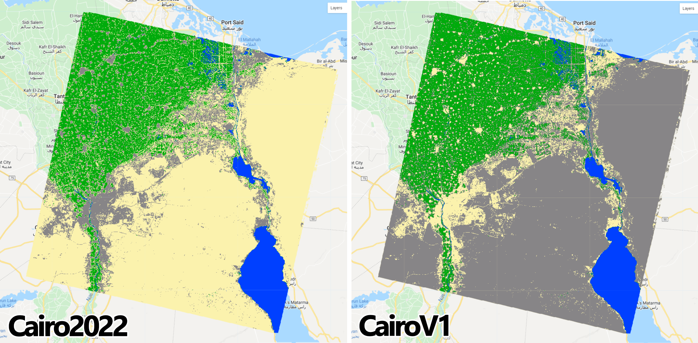
Figure 1.72: Cairo2022 and CairoV1 maps using the original paletteMap. Note that Sand and bare areas and Built-up and Urban areas switched colors as we switched their order.
*Scenario 2
A new version of the Cairo2022 map where Sand and bare areas (pixel value = 2) and Built-up and Urban Areas (pixel value = 3) are merged into a new class called Barren land and Articicial Surfaces (pixel value = 2). Note that this new class can assume any value when merging, as long as both classes have the same value:
Figure 1.73: Sand and bare areas merging with Built-up and Urban area into a new class value (2). New classes can assume any value when merging, as long as these values are the same for both classes.
For this example, we will keep the value 2 for this new class in a new variable CairoV2 for the new map:
var CairoV2 = Cairo2022.remap([0,1,2,3],[0,1,2,2]);We will add the CairoV2 to the the map using the original color scheme paletteMAP.
Map.addLayer(CairoV2, {min: 0, max: 3, palette:paletteMAP}, 'Cairo V2');
Note that the min and max range of values changed from 0-3 (4 classes) to 0-2 (three classes) in CairoV2. You can still maintain the original min and max range of values in this particular case because Map.addLayer() would only map the color scheme to the first three values ofCairov2 (0, 1 and 2). However, it is always good practice to set the min and max range of values to match the actual number of classes along with editing the color palette to have the same number of colors as the number of classes in your map.
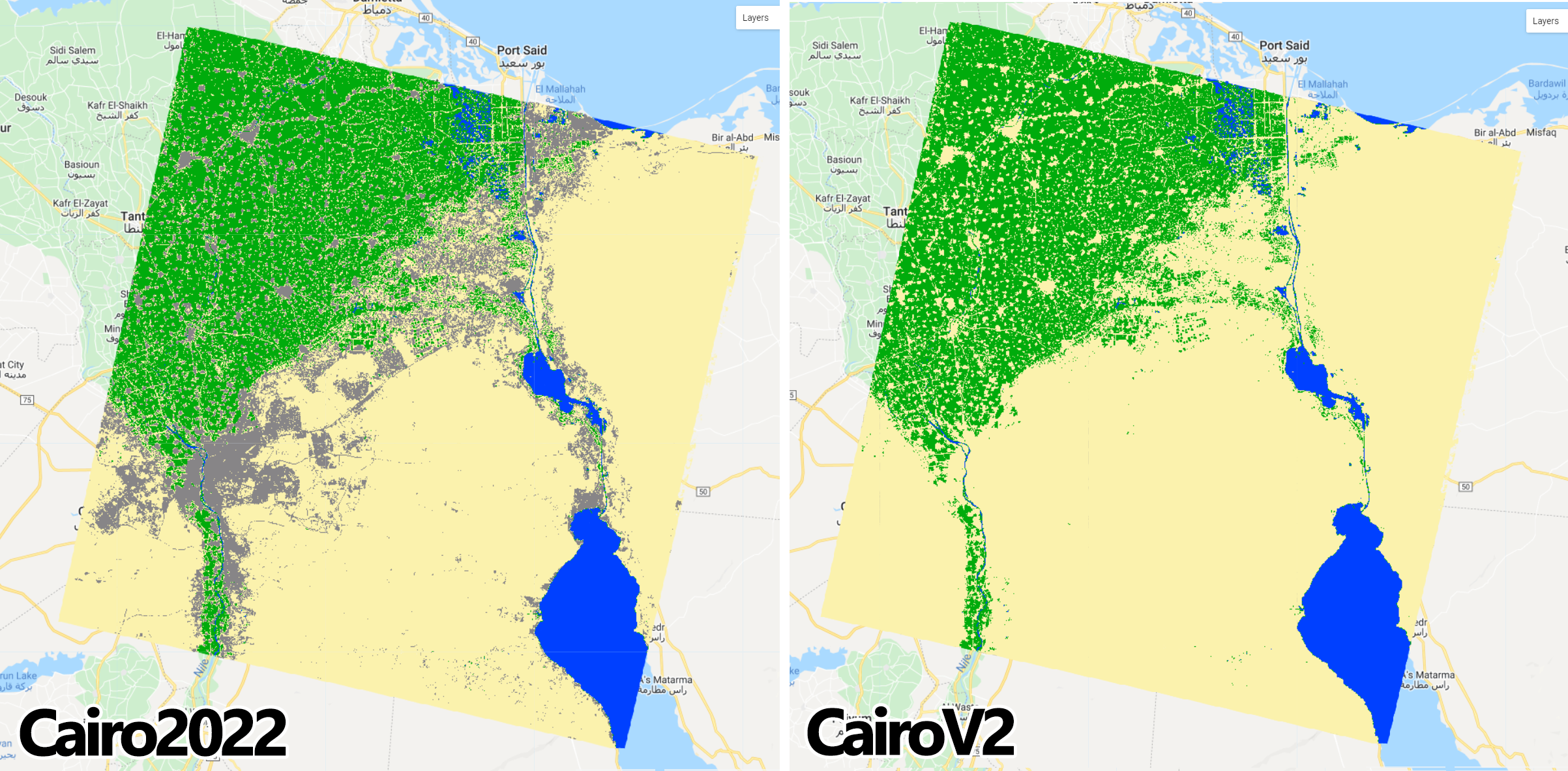
Figure 1.74: Cairo2022 and CairoV2 maps using the original paletteMap. Note that Sand and bare areas and Built-up and Urban areas have the same color as they were merged under the same pixel value (2).
*Scenario 2
A new version of the Cairo2022 map where only a portion of it is remapped to a given class. This scenario is one of the most commonly used post-classification procedure where the goal is to remap specific areas to fix for classification errors. To ilustrate, we will consider the following example:
Upon close inspection, the Cairo2022 map showed some cropland/cultivated areas within zones of dense urbanization of New Cairo City. A team on the ground went to the area and confirmed that is indeed dense urbanization and no agricultural land was found in that area. Therefore, that portion of the map needs to be rectified in order to reflect the actual land cover. In this case, the .where() method of an ee.Image() object is used. This function performs conditional replacement of values, following the formula input.where(test,value). For each pixel in each band of input, if the corresponding pixel in test is nonzero, Google Earth Engine will output the corresponding pixel in value, otherwise it will output the input pixel. Translating this function to this example, input is the land cover map in which we aim to perform the reclassification - in this case Cairo2020; test is the area or region of the map value will take place, and; value is the correct classification that will be included in the final map:
Figure 1.75: The .where function applied to this example.
In your own version of Cairo2022 map, create an new geometry over an area of your interest and name it aoi:
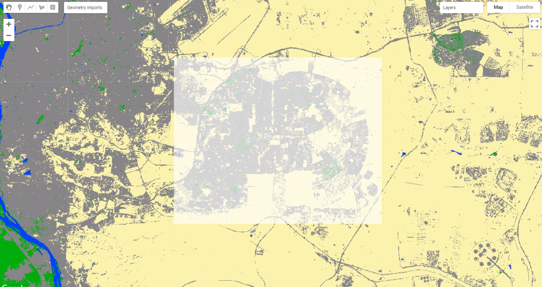
Figure 1.76: A geometry over an area of Cairo2020 highlighting cultivated areas next to urbanization.
The method .where() only uses ee.Image() objects as test. Therefore, using the geometry/feature aoi is not allowed. An easy and effective way to go around this rule is to create an image with ee.Image() and clip it for the region of interest:
var region = ee.Image(1).clip(aoi);The function above will create an image with value of 1 and will clip it for the area of interest aoi. Next, using the same approach from Scenario 1 and 2, we will create a new version of Cairo2022 called ''subistitute', where the Cropland/Cultivated Areas class is remapped to Built-up and Urban Areas: the position 2 on list 2 (belonging to agricultural/cultivated areas) receives the value 3 from Built-up and Urban Areas on list 1:
var substitute = Cairo2020.remap([0,1,2,3],[0,3,2,3]);Now, using .where() we will create a new map CairoV3 following the formula (1.75) and add it to the map editor:
var CairoV3 = Cairo2022.where(region,substitute);
Map.addLayer(CairoV3, {min: 0, max: 3, palette:paletteMAP}, 'Cairo V3');
Compare the two classification objects: you will notice that every pixel of Cropland/Cultivated Areas (green, pixel value = 2) within the aoi in Cairo2022 is now remapped to Built-up and Urban Areas (grey, pixel value = 3) in CairoV3:
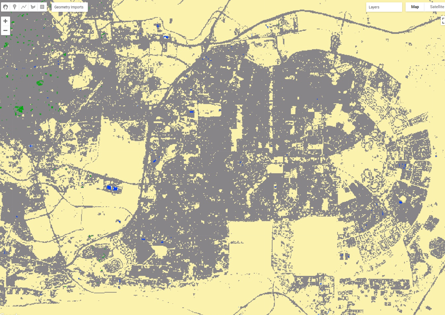
Figure 1.77: CairoV3 showing the pixels of Cropland/Cultivated Areas remapped as Built-up and Urban Areas within aoi.
1.4.2 Map spatial smoothing
Spatial smoothing is another post-classification procedure to enhance the quality of a land cover classification output. A common issue that arises from the pixel-based classification of fine/medium spatial resolution imagery is the “salt-and-pepper” effect. This happens when individual pixels are classified differently from their neighbors, creating speckles of isolated pixels of different classes. There are several ways to minimize this issue, such as:
image pre-processing, such as low-pass filter and texture analysis;
contextual classification, and;
post-classification processing, such as median and mode filtering.
In this section, we will focus on a post-classification technique to reduce the salt and pepper effect and edge roughness of land cover maps using focal median filtering (ee.Image.focal_median()).
We will apply the .focal_median() method to Cairo2022. This method is a simple sliding-window spatial filter that replaces the center value (or class) in the window with the median of all the pixel values in the window. The window, or kernel, is usually square but can be any shape. The .focal_median() method usually is expressed as:
Figure 1.78: .focal_median spatial filter.
In the function above, the radius parameter specifies the number of pixels from the center that the kernel will cover. This radius value can be expressed as number of pixels or meters. The kernelType specifies the type of kernel to use.
Either .focal_median(1, 'square', 'pixels') or .focal_median(30, 'square', 'meters') will produce a 3x3 pixel sliding-window, as you are specifing 1 pixel (or 30 meters which is equal to one Landsat pixel) in each direction from the center pixel. Similarly, a radius of 2 pixels or 60 meters will produce a 5x5 sliding-window: a center pixel plus 2 pixels in each direction.
Following Figure 1.78 and the example above, we will apply the .focal_median() filtering with two radius sizes (30 and 60 meters) to Cairo2022, add Cairo30 and Cairo60 to the map editor and compare the results:
var Cairo30 = Cairo2022.focal_median(30,'square', 'meters');
var Cairo60 = Cairo2022.focal_median(60,'square', 'meters');
Map.addLayer(Cairo30, {min: 0, max: 3, palette:paletteMAP}, 'Cairo 3x3');
Map.addLayer(Cairo60, {min: 0, max: 3, palette:paletteMAP}, 'Cairo 5x5');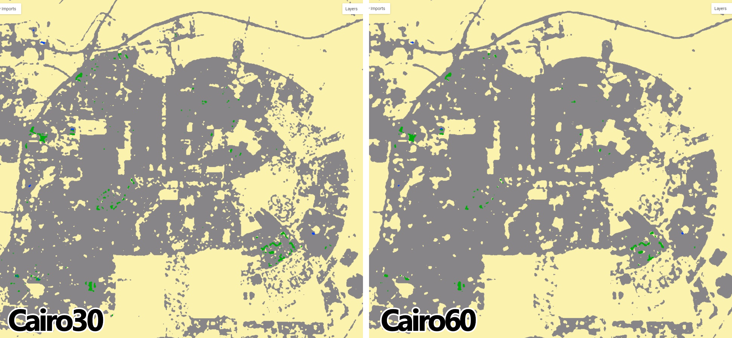
Figure 1.79: Cairo2022 processed with .focal_median spatial filter two radius sizes.
IMPORTANT: The .focal_median(1, 'square', 'pixels')* and .focal_median(30, 'square', 'meters') will only achieve the intended final result if you reproject it back to the original scale and projection from the original map. Note that this technique while effective in removing the "salt-and-pepper" effect from the original map, it creates edges that are not in the same resolution and projection as the original map. Therefore, creating fairly rounded boundaries for the classes. This is not ideal as it is usually intended for these maps to keep the same resolution as the original map, as well as to preserve the boundaries between classes. To account for this issue, you can reproject this output back the original scale so it is formed by 30 x 30 meter pixels. To do that, simply use .reproject(projection.atScale(scale)) within the .focal_median filter. The .reproject function will take two arguments: projection and scale. You can extract this information from the original map with .projection() and .nominalScale():
var projection = Cairo2022.projection();
var scale = projection.nominalScale();
Then, we re-aply the .focal_median() filter with .reproject(projection.atScale(scale)):
var newCairo30 = Cairo2022.focal_median(1,'square', 'pixels')
                       .reproject(projection.atScale(scale));

var newCairo60 = Cairo2022.focal_median(60,'square', 'meters')
                       .reproject(prj.atScale(scale));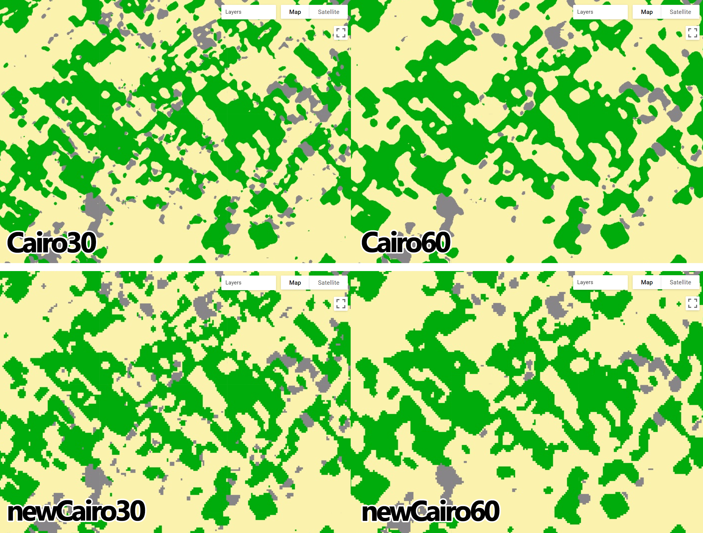
Figure 1.80: Cairo2022 processed with .focal_median spatial filter with 3x3 and 5x5 pixel windows. Note that the function was reprojected to match Cairo2022's projection and scale. Now the discrete boundaries of classes are pixelated back to 30 meters.
Note that even though the boundaries of the classes are smoother, they are formed by the 30 x 30 meter pixels. Usually, a radius of 1 (3x3 square window) removes most of the salt-and-pepper effect, smoothens the boundaries in between classes while preserving the overall shape of the classes.
Access the full scrip for this section here.
Reflectance is the ratio of the amount of light leaving a target to the amount of light striking the target. It has no units.